Heathkit IT-3121 — Vol 2: How a Semiconductor Curve Tracer Works

2.1 The one idea behind every curve tracer

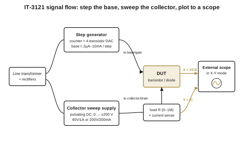
A curve tracer answers a question no meter can: what does this device’s output current do as I sweep the voltage across it — and how does that answer change as I vary the input drive? A DMM gives you one operating point at a time; a curve tracer gives you the whole surface. To do it, the instrument runs three things simultaneously and lets the scope superimpose the results:

1. It sweeps the main terminal voltage — collector, drain, or anode — from zero up to some peak and back, over and over, a hundred-odd times a second.
2. It steps the control input — base current for a bipolar transistor, gate voltage for a FET — through a staircase of precisely known values, holding each one for a full sweep.
3. It plots the device’s output current (vertical) against the swept terminal voltage (horizontal) on an X-Y display.

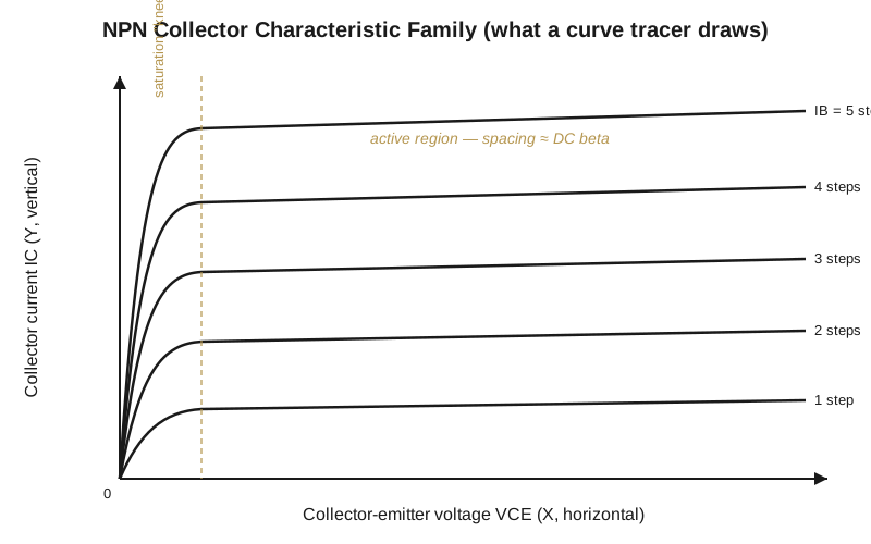
Sweep once and you get one curve — the device’s I-V characteristic at a single drive level. Step the drive up one notch and sweep again, and a second curve lays itself down above the first. Do it for a handful of steps and the display holds the whole family of characteristic curves: the transistor’s fingerprint. Because the sweep is fast and repetitive and the staircase recycles, the family sits there as a stable, glowing figure you can read, adjust, and compare against another device in real time.

The IT-3121 does exactly this with late-1970s analog hardware and nothing else. Erickson, who reverse-engineered the design for his modern clone (Vol 3), counts the whole parts list as “18 transistors, 5 ‘741 Opamps, one TTL counter,” with “the magic in the transformer and the switching.” There is no microprocessor, no CRT, and no software — every function in the three-step recipe above is a discrete-transistor or op-amp block, and the display is a scope you already own. That austerity is exactly what makes the IT-3121 the clearest possible machine to learn the principle on: each block does one legible thing.

2.2 The swept collector supply

The horizontal axis is the voltage across the device under test, and the IT-3121 generates the sweep the cheap, clever way every vintage tracer did: it does not synthesize a regulated ramp — it uses the raw shape of rectified mains as the sweep. The line transformer’s secondary is rectified into pulsating DC, so the collector voltage naturally climbs from zero to a peak and falls back to zero once per rectified mains hump — a rate tied to the line frequency (tens of times a second; the exact figure depends on whether the rectifier is half- or full-wave, which the primary manual/schematic would settle). Each of those rising humps is a voltage sweep from 0 to V-peak, complete with a built-in retrace to zero at the crossing. The power line hands you a free, repetitive, self-retracing 0-to-max ramp at exactly the refresh rate the eye wants.

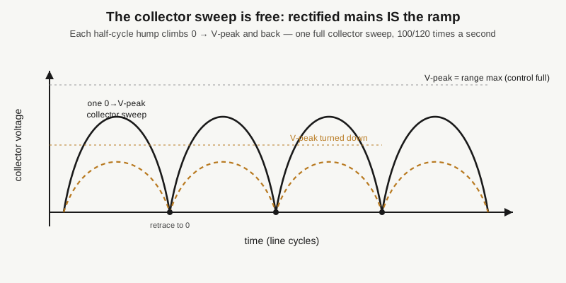
A front-panel voltage control sets how high each hump reaches, dialing the sweep from a few volts up to the range maximum. There is nothing exotic downstream of it — a pass/buffer stage carries the current to the device — but the important part is conceptual: because the ramp is the mains waveform itself, the tracer never has to make a sweep, only limit its amplitude. Turn the control down and every hump gets shorter; the device simply gets swept over a smaller slice of voltage.

Two ranges cover the operating envelope, and the split matters:

• 40 V at up to 1 A — the low-voltage, high-current range. This is for pushing serious current through power transistors and rectifiers, where you care about saturation behavior and current handling, not high voltage. The 1 A ceiling is available only here.
• 200 V at up to 200 mA — the high-voltage, low-current range. This reaches the breakdown and avalanche voltages of higher-voltage parts, at currents kept modest so nothing cooks.

So the collector supply’s absolute limits are ±200 V (on the 200 V range) and 1 A (on the 40 V range) — and those two maxima never occur together. It is worth carrying that as a bench fact: the “±200 V” that governs your safety habits belongs to the low-current range; the ampere belongs to the low-voltage range. Erickson, sizing his redesign against the original, summarizes the whole envelope as “collector voltage up to +/- 200V and currents up to 1A with simple controls and lots of ranges” — and elsewhere flags that ±200 V is “low for some devices, particularly tubes,” which is why the same architecture stretched to tube work wants far higher rails. For the semiconductors the IT-3121 was built to trace, ±200 V is plenty.

2.2.1 Series limiting resistance and the load line

Every curve tracer of this kind puts some series resistance between the swept supply and the device under test — this is a general principle of the architecture, and how the IT-3121 specifically sets it (fixed with range, or a separate control) is a detail the primary manual would settle. Whatever its exact implementation, that series resistance does two jobs at once:

• Protection / current limit. If the DUT conducts hard — a saturated power transistor, or a diode past its knee — series resistance caps how much current can flow, protecting both the device and the instrument. A high-current range wants a small resistance; a high-voltage range driving a small-signal part wants a large one so only a milliamp or two ever flows.
• Load line. The series resistance sets the slope the device works against. The collector voltage the DUT actually sees is the supply peak minus the drop across that resistance, so as the device draws current the operating point slides down a straight line whose slope is set by the resistance — the classic load line laid over the characteristic family. Reading where that line crosses each curve is how you locate saturation and cutoff, which Vol 4 works through on a live device.

Between them, the voltage control sets how far right the sweep reaches and the range sets the voltage/current envelope; the series limiting resistance governs how steeply current is allowed to build as the device turns on.

2.3 The stepped base/gate drive

The other input to the picture is the control drive — and this is where a curve tracer earns its name. It does not apply one drive level; it marches through a staircase of them, so every collector sweep is taken at a different, precisely known input. The verified generation path in the original is a TTL counter clocking a staircase generator: the counter counts up, the staircase advances one tread per count, and after the top step it resets and starts over. That counter is the “one TTL counter” in Erickson’s parts tally, and it is the only piece of digital logic in the whole instrument.

2.3.1 Bipolar transistors: a constant-current staircase

For a bipolar transistor the controlling quantity is base current, not voltage — collector current is set by base current through beta, and base voltage would be a treacherous knob because of the exponential diode relationship at the base-emitter junction. So the IT-3121 drives the base from a constant-current step generator: each tread of the staircase is a fixed number of microamps or milliamps of base current, independent of what the base-emitter voltage happens to settle at.

The step-amplitude switch selects the size of each tread over a wide range — 0.002 mA to 10 mA per step, i.e. 2 µA/step up to 10 mA/step, in a 1-2-5 sequence (2 µA, 5 µA, 10 µA, 20 µA, … 5 mA, 10 mA). A separate control sets how many treads appear in the staircase. So a setting of “0.1 mA/step, 5 steps” tells the instrument to trace five curves, at base currents of 0.1, 0.2, 0.3, 0.4, and 0.5 mA.

That known, uniform spacing is the entire point. Beta is the change in collector current per change in base current:

$$\beta_{DC} = \frac{I_C}{I_B}, \qquad \beta_{AC} = \frac{\Delta I_C}{\Delta I_B}$$

Because every tread advances base current by the same known amount, the vertical distance between adjacent curves, divided by the step size, reads out as beta directly — no separate measurement, just a count of divisions on the scope graticule. A worked example: on the 0.1 mA/step setting, if two neighbouring curves in the flat active region sit 5 mA of collector current apart (read from the scope’s current-per-division), then ΔI_C / ΔI_B = 5 mA / 0.1 mA = beta ≈ 50. Evenly-spaced curves mean constant beta; curves that bunch up at the top mean beta falling off at high current — you see the gain compress. This is precisely the reading Erickson gets on his first real device in the clone (Vol 3): a 1970s D44C9 NPN power transistor driven at 200 µA/step, curves spaced to give “Beta … about 50.” (Keep that figure straight from a different early bench test of his — a 100 µA/step drive into a 1 kΩ resistor — which was a bring-up sanity check of the step generator itself, not a transistor measurement; the two share nothing but a family resemblance.)

2.3.2 FETs: a voltage staircase instead

A field-effect transistor is voltage-controlled — the gate draws essentially no current, and drain current is governed by gate-source voltage. A current staircase would be meaningless. So for FETs the step generator switches modes and produces a voltage staircase of 0.05 V to 1 V per step (again 1-2-5). Now each curve corresponds to a known gate-source voltage, and the vertical spacing reads out transconductance (g_m = ΔI_D / ΔV_GS) the same way base-current spacing read out beta. The original handles JFETs, both N- and P-channel; it does not natively do enhancement-mode MOSFETs — those need a positive gate offset the stock step generator can’t supply, which is why a MOSFET capability shows up only as an aftermarket op-amp offset board (a documented breadboard mod) or as a designed-in feature of Erickson’s redesign (Vol 3).

2.3.3 Diodes: the degenerate case

A two-terminal part — an ordinary diode, a zener, a tunnel diode — has no control terminal, so there is no staircase at all. You sweep the collector supply across the single junction and read one curve: the forward knee, the reverse leakage, and, on the 200 V range, the reverse breakdown or zener voltage where the curve slams vertical. A tunnel diode even shows its negative-resistance dip. The stepped drive simply sits idle; the swept supply and the X-Y plot do all the work.

2.3.4 Polarity and the four quadrants

A single polarity switch flips the step generator and the collector supply together, so the whole picture reflects into the correct quadrant of the X-Y plane. NPN and N-channel parts trace up-and-to-the-right (positive collector voltage, positive collector current); PNP and P-channel parts want negative drive and trace into the opposite quadrant. Ganging both polarities on one switch is what lets the same instrument handle complementary parts without rewiring — and it is what makes matched-pair checking trivial: trace an NPN, flip polarity, trace its PNP complement, and compare the two families against the same graticule.

2.4 The timing that makes the family coherent

Here is the subtlety worth internalizing, because it is what keeps the curves from smearing into each other:

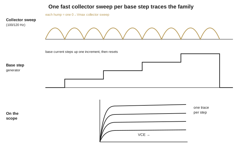
The collector sweeps fast — the mains-derived ramp, recurring at a multiple of the line frequency — while the base staircase advances slowly, holding each tread long enough for at least one clean collector sweep before it increments. Each step therefore paints exactly one curve; when the staircase reaches its top it resets to zero and the whole family repeats. Because the entire cycle recurs many times a second, persistence of vision fuses the sequence into one steady figure even though, at any instant, the beam is drawing only a single curve at a single base current. Get the timing relationship backwards — sweep slow, step fast — and you would draw garbage; the fast-sweep / slow-step hierarchy is the quiet reason the family holds still.

2.5 Turning current and voltage into X and Y

The scope is a two-axis voltmeter, so the IT-3121’s last job is to hand it two voltages, each proportional to a quantity you care about, and let the scope’s own graticule serve as the measuring grid.

• X (horizontal) — collector voltage. This is simply the actual voltage across the device’s main terminals — collector-emitter, or drain-source — buffered out to a banana jack. A voltage-sensitivity switch scales it so a chosen number of volts equals one scope division. X is the swept quantity, so the horizontal extent of the trace is the voltage range the device saw.
• Y (vertical) — collector current. Current is not directly a voltage, so the instrument reads it as the small voltage developed across a current-sense resistor in the collector/drain return path, then a current-sensitivity switch scales that to so-many milliamps per division. Y is the device’s response, so the vertical excursion of each curve is how much current flowed.

You put the scope in X-Y mode, feed X and Y from the IT-3121’s banana jacks into the scope’s horizontal and vertical inputs, and read the family directly against the scope’s graticule: horizontal grid lines are volts-per-division as the front-panel switch says, vertical lines are milliamps-per-division as its switch says. There is no calibrated internal graticule the way a self-contained Tektronix 575/576 has — the scope you already own is the display, and offloading the CRT is exactly the trade that made the IT-3121 the affordable hobby-and-service tracer rather than a benchtop the size of the Tek (see Vol 1 for where it sits in the line, and why its electrically-identical older twin the IT-1121 exists). The cost is a small loss of convenience — you calibrate your reading to the scope’s graticule, not a dedicated one — and the payoff is a tracer a hobbyist could actually afford.

2.6 What each front-panel control does, mapped to the block diagram

Pulling the operator’s controls together against the story above, so the panel stops being a wall of knobs and reads as the block diagram it implements:

Table 1 — Pulling the operator's controls together against the story above, so the panel stops being a wall of knobs and reads as the block diagram it implements

Control	Block it drives	What it sets
Collector range switch	swept supply	selects the operating envelope: 40 V / 1 A (high-current) vs 200 V / 200 mA (high-voltage)
Collector voltage control	swept supply	peak of the swept collector supply, 0 → range max (how far right the sweep reaches)
Step amplitude switch	step generator	base current per step (2 µA – 10 mA/step) or, in FET mode, gate volts per step (0.05 – 1 V/step)
Number of steps control	step generator	how many curves appear in the family
Polarity switch	step gen + supply together	NPN/PNP, N-/P-channel — reflects the whole picture into the correct quadrant
Current sensitivity switch	Y output	vertical scaling — collector current per scope division
Voltage sensitivity switch	X output	horizontal scaling — collector voltage per scope division
X, Y outputs	to external scope	banana jacks to the scope’s X-Y inputs

Every one of those controls lands on a piece of the three-step recipe: two shape the collector sweep, two shape the base/gate staircase, one sets polarity, and two scale the axes. Understand the block diagram and the panel reads itself.

That is the architecture end-to-end: step the base or gate through a known staircase, sweep the collector with free rectified mains, sense the current, and hand X and Y to a scope in X-Y mode. Vol 3 picks up what a modern designer keeps and what he throws away when he rebuilds this same architecture around a microcontroller, a DAC, and relays instead of a TTL counter and expensive rotary switches — and what breaks first on a forty-year-old original. Vol 4 is the sit-down-and-drive-it procedure: wiring it to a scope, running a device, reading gain and breakdown off the graticule, and staying clear of that ±200 V supply.