VBA Curve Tracer — Vol 2: How It Works — Principle and Circuit Design

2.1 The sweep-and-step principle

Every analog curve tracer, from a 1960s Tektronix 575 to Paul Versteeg’s VBA, is built on one idea: to draw a component’s current-versus-voltage characteristic you drive the part with two coordinated sources and read back two quantities, then plot one against the other instead of against time. Strip away the packaging and the machine is four functional pieces — a swept source, a stepped source, two measurement channels, and a display that plots X against Y. The VBA implements all four in hardware, with no digitiser and no processor anywhere in the signal path.

2.1.1 What a family of output curves is

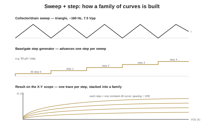
Take a bipolar transistor. Its output characteristic is the collector current (I_C) plotted against the collector-emitter voltage (V_{CE}), for a fixed base drive. Hold the base current at, say, 50 µA and sweep (V_{CE}) from zero upward: the collector current climbs steeply out of saturation, then flattens into the active region where it is nearly independent of (V_{CE}). That single flat-topped trace is one curve. Now repeat it at 100 µA, 150 µA, 200 µA, and so on. Each base level draws its own curve, and because a higher base current commands proportionally more collector current, the curves stack into a fan. The vertical spacing between adjacent curves is the current gain — a wide fan means high (h_{FE}), a compressed fan means low gain. Read the same picture a different way and it also gives you the output resistance (the residual upward slope in the active region), the saturation voltage (how far right the knee sits), and the breakdown voltage (where the far-right end of a curve suddenly bends upward). One image, several parameters. That density of information is why the curve tracer never went away.

The same construction works for every device the VBA targets. For a MOSFET the swept terminal is drain-source and the stepped terminal is the gate voltage; for a diode there is no stepped terminal at all, just a single swept trace of forward and reverse current versus voltage. The engine underneath does not change — only what you connect to the swept and stepped outputs.

2.1.2 Sweep: the swept main-terminal voltage

The horizontal axis is the device’s own terminal voltage, and it has to be swept — driven repeatedly from zero to a maximum and back — fast enough that the eye sees a solid line rather than a moving dot. The VBA generates this as a triangle waveform whose frequency is adjustable over roughly 140 Hz to 650 Hz. At 140 Hz a full up-and-down sweep takes about 7.1 ms; at 650 Hz it takes about 1.5 ms. That band is chosen for a reason at each end. Too slow and the trace flickers and the device sits at high dissipation longer per sweep; too fast and the device’s own capacitances and the measurement amplifiers start to smear the trace, because at high sweep rate the (C,dV/dt) displacement currents in and around the part become a measurable fraction of the current you are trying to read.

2.1.3 Step: the stepped control-terminal drive

The second source produces the family. It holds a control-terminal level constant for exactly one sweep, then advances to the next level, so that each level paints one complete curve before the next begins. The VBA’s step generator produces 0 to 7 steps — that is up to eight traces on screen counting the zero-current step. The magnitude of each step is selectable in a 1-2-5 sequence spanning an enormous range, from 5 V / 5 mA per step at the coarse end down to 50 µV / 50 nA per step at the fine end. The coarse end drives power transistors that want milliamps of base current per curve; the fine end resolves the picoamp-class gate leakage and threshold detail of small-signal FETs. A Polarity control flips the whole staircase between positive-going steps (for N-type devices) and negative-going steps (for P-type), and an Offset control shifts the staircase’s starting point — nominally ±2 V, or ±10 V with an optional modification — so that FET families can be centred on the threshold voltage rather than forced to start at zero.

2.1.4 Why the two sources must be synchronised

The step generator must advance in lockstep with the sweep, and the transition must land at the bottom of a sweep, not partway up one. If a step changed mid-sweep, that curve would show a discontinuity — the trace would jump from one gain line to another halfway across the screen. So the timing is: one sweep, one step; one sweep, one step. There is also an optional dwell inserted between steps — the front-panel Step Delay, adjustable over roughly 40 ms to 250 ms — which does nothing for the picture and everything for the device. At high dissipation the die heats during each sweep; holding a step for an extra fraction of a second lets it cool before the next curve is drawn, which is the difference between reading a power transistor’s true characteristic and cooking it. With eight active steps and no added delay a whole family refreshes at the sweep rate divided by eight — roughly 17 to 80 families per second across the frequency band — fast enough to look solid. Dial in 250 ms of step delay and each step alone takes a quarter-second, so a full eight-step family now takes on the order of two seconds to paint: slow, deliberate, and thermally safe.

2.1.5 Why a triangle, and why fully analog

Two design choices define the VBA’s character. The first is the shape of the sweep: a triangle, not a rectified half-sine. A linear ramp maps directly and undistorted onto the scope’s horizontal axis, so a volt on the device is a fixed number of screen divisions regardless of where in the sweep you are — a rectified sine, by contrast, crowds the trace at the ends and stretches it in the middle. The linear ramp also spends equal time at every voltage, which spreads the device’s dissipation evenly across the sweep instead of dwelling at the peaks the way a sine does.

The second choice is that the instrument is fully analog end to end. There is no microcontroller and no PC-side software anywhere in it. The tracer emits two buffered analog voltages — device voltage on one BNC, device current on another — and an oscilloscope in X-Y mode is the display. In X-Y mode the scope abandons its time base and plots channel-1 deflection against channel-2 deflection, which is exactly the I-V plot you want: feed it “device voltage” on X and “device current” on Y and the beam traces the curve directly, in real time, with no sampling, no frame buffer, and no host in the loop. Paul Versteeg drove the writeup’s screenshots from a Rigol DSO in X-Y mode, but any analog CRT scope with an X-Y setting works identically — and on a CRT the response is genuinely instantaneous. The all-analog approach is what gives the VBA its live feel: turn a knob and the curve moves now, with none of the latency a digitise-process-redraw pipeline imposes. It is the same philosophy that made the classic Tektronix tracers a pleasure to use, rebuilt from modern parts.

2.2 The VBA’s analog architecture

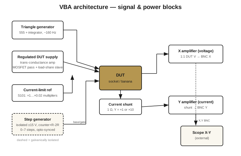
Functionally the instrument is five blocks: a triangle-sweep generator, a regulated DUT supply with its current limiter, a step generator that floats on the device’s control terminal, a pair of X/Y measurement amplifiers, and a multi-rail power supply feeding them all. Those five blocks are physically distributed across four printed-circuit boards — a Main board and a Front board carrying the active circuitry, plus a Front-panel board and a Back-panel board carrying the controls and connectors. The board-level partitioning and the build itself are Vol 3’s subject; here the concern is what each block does and why it is built the way it is.

2.2.1 The triangle-sweep generator

The sweep is a triangle whose frequency is adjustable across the 140–650 Hz band. The standard way to generate a linear triangle like this is an integrator wrapped in a loop with a comparator: the integrator charges a capacitor at a constant rate to produce a linear voltage ramp; when the ramp reaches the comparator’s upper threshold the comparator flips, reverses the integrator’s input, and the ramp runs linearly back down until it hits the lower threshold, whereupon the comparator flips again. The result is a clean, symmetric triangle whose slope — and therefore its frequency — is set by the integrating capacitor and the charge current, which is what makes the frequency adjustable. (The VBA’s exact sweep circuit, and how its frequency and its turning-point alignment with the step transitions are actually trimmed, aren’t detailed in the published writeup — confirm against Versteeg’s schematic before quoting specifics.)

2.2.2 The regulated DUT supply

This is the heart of the machine and the block that Bud Bennett’s circuit-development work shaped most. Its job is brutal: take the triangle from the sweep generator and reproduce it faithfully across the device under test — but at real power, sourcing up to 2 A, while also standing ready to limit current the instant the device demands more than the front-panel setting allows.

It does this with a linear series-pass regulator built around power MOSFETs. Linear, not switching, because a switcher’s ripple and its finite loop bandwidth would corrupt a waveform that has to stay clean from DC to a few hundred hertz and act as both the source and the reference for the horizontal axis. The pass MOSFETs drop the difference between the raw supply rail and the device voltage, and that difference times the device current is dissipated as heat in the passing device — which at 2 A on the low-voltage range is real wattage. The pass devices are consequently mounted on large heat-sinks; the design uses more than one pass MOSFET so the dissipation is shared rather than concentrated in a single junction.

The regulator’s defining trick is a graceful handover between constant-voltage and constant-current operation. When the device is happily following the swept voltage, the loop is in constant-voltage mode: it forces the device terminal to track the triangle. The moment the device tries to draw more than the current setting — because a transistor has entered saturation, or a diode has gone into hard conduction, or something has shorted — the loop transfers control to the current-limit path and holds the current at the set ceiling while letting the voltage fall to whatever the device imposes. On a curve this is exactly the behaviour you want: the trace runs up the constant-voltage wall and then turns cleanly along the constant-current ceiling, with no overshoot, no oscillation, and no glitch at the corner. A naive op-amp regulator slammed into its limit tends to stick, ring, or hiccup at that transition; getting the corner clean is the hard part of the design, and it is where the linear-design experience in the “B” of VBA earned its place.

2.2.2.1 The three envelopes

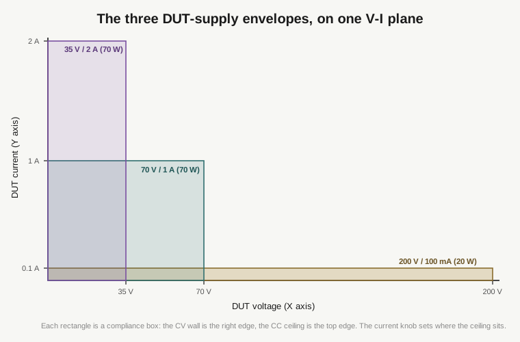
The supply offers three voltage/current ranges, and they are genuinely distinct operating envelopes rather than one range scaled three ways:

• 0–35 V at up to 2 A — the high-current, low-voltage range, for power transistors and anything you want to push into real conduction.
• 0–70 V at up to 1 A — the mid range, the general-purpose setting for most small- and medium-power work.
• 0–200 V at up to 100 mA — the high-voltage, low-current range, for breakdown and reverse-characteristic tests.

Notice the trade the three envelopes encode: the two lower ranges peak at about the same corner power (35 V × 2 A and 70 V × 1 A are both ≈ 70 W), while the 200 V range deliberately backs the current off to 100 mA (≈ 20 W) because standing off 200 V across the pass device leaves far less headroom for dissipation. The 2 A ceiling is what caps high-current work and the 200 V ceiling is what caps high-voltage breakdown testing — and, notably, 200 V is not enough for most vacuum tubes, which is where the tube-oriented tracers in this category (the uTracer and eTracer families) take over from the VBA.

2.2.2.2 Current limiting and the six multipliers

The current ceiling in that picture is not fixed at the range maximum — it is continuously and precisely settable, which is what lets you protect a fragile part or zoom the vertical axis onto a small current. The limit is derived from a stable reference that the front-panel Current range switch scales down in fixed ratios, giving six multipliers: ×1, ×0.5, ×0.2, ×0.1, ×0.05, and ×0.02. On the 2 A range those multipliers set full-scale current limits of 2 A, 1 A, 400 mA, 200 mA, 100 mA, and 40 mA respectively. (Whether the same ratios rescale to each of the other ranges’ own current maxima is the natural expectation, but the published sources confirm only the ratios themselves and this 2 A worked case — check the blog/BOM before relying on the per-range figures.) Choosing a lower multiplier does two things at once: it caps how much current the device can draw (protection) and it sets the vertical sensitivity of the plot (resolution), because the current-sense signal is referenced to that same full-scale figure.

2.2.3 The reservoir capacitor and range switching

Between the mains transformer and the linear regulator sits a reservoir capacitor that smooths the rectified raw DC and, just as importantly, absorbs the transient that occurs when you switch voltage ranges — reconfiguring the supply’s raw rail on the fly would otherwise throw a spike at the pass device and the DUT. On the low- and mid-voltage ranges an ordinary electrolytic handles this. The 200 V range is the interesting one, because 200 V is above the comfortable rating of common high-value electrolytics. Versteeg’s solution is not a single exotic high-voltage part but two 1,000 µF / 100 V electrolytics wired in series. Two 100 V capacitors in series stand off roughly 200 V between them, at the cost of halving the capacitance to about 500 µF — the standard series-stacking trade of voltage rating for capacitance. (Series-stacked electrolytics normally want balancing resistors across each cap so the DC voltage divides evenly and neither part is over-stressed; that is the conventional accompaniment to this arrangement.) The point worth fixing in memory: the 200 V reservoir is two series 1,000 µF / 100 V caps giving ~200 V and ~500 µF, not a single high-voltage part.

2.2.4 The step generator

The step generator builds the staircase that produces the family of curves. Once per sweep it advances by one increment, producing a clean, evenly spaced staircase whose height per step is set by the front-panel range in the 1-2-5 sequence described earlier (5 V / 5 mA down to 50 µV / 50 nA). (The exact circuit that generates the staircase — whether a counter driving a resistor-ladder DAC or some other scheme — isn’t spelled out in the published writeup; read Versteeg’s schematic before quoting a topology.) The Steps control sets how many steps are active, 0 through 7; Polarity sets the staircase’s direction for N- or P-type devices; Offset biases the whole staircase up or down; and Step Delay inserts the between-steps dwell for thermal relief.

For a bipolar transistor the step output is used as a base current source — each step is a fixed increment of base current — while for a MOSFET or JFET the same output is used as a gate voltage source, each step a fixed increment of (V_{GS}). That the step generator can be either a current source or a voltage source, positive- or negative-going, offset either way, is what lets the one instrument trace NPN and PNP bipolars, N- and P-channel MOSFETs, and depletion-mode JFETs that need the staircase parked in negative gate-voltage territory.

There is a subtle architectural requirement hiding in all of this. The step drive is referenced to the device’s control terminal, which sits at whatever potential the swept main terminal has driven the device to — it does not sit at the instrument’s ground. To drive a stepped current or voltage into a terminal that is itself floating on the sweep, the step generator must run from a supply that floats along with it, galvanically separated from the ground-referenced sweep and measurement circuitry. This isolated, floating step supply is what makes it possible to drive both device polarities and to reference the steps correctly against the moving main-terminal voltage; it is also what keeps the low-level base/gate drive from being contaminated by ground currents flowing in the high-current DUT supply.

2.2.5 The X/Y measurement path

Two things have to be measured and handed to the scope: the device’s voltage (the X axis) and the device’s current (the Y axis).

Device current is sensed as a voltage in series with the device — the usual curve-tracer arrangement, though the VBA’s exact sense element isn’t detailed in the published writeup. That sense voltage is buffered and scaled by a Y amplifier before it leaves the instrument, and device voltage is buffered by an X amplifier; the writeup doesn’t state either amplifier’s gain, so any specific gain figure (or a ×1/×10 sensitivity switch, as some tracers carry) should be read off Versteeg’s schematic before it is quoted. What is documented is that the plot’s vertical sensitivity is set by the six current multipliers (×1 down to ×0.02) referencing the current-sense signal to the selected full-scale figure. Both amplifiers drive back-panel BNC connectors straight into the scope’s X and Y inputs. This is also where the instrument’s limits meet the display’s limits: at the finest current settings the useful resolution is bounded not by the tracer but by the noise floor of whatever scope is reading it — a DSO cranked to 100 µV/div is reading its own noise as much as the device’s, which is why the low-level ranges reward a quiet analog CRT.

2.3 Power and packaging

The five signal blocks all draw from a common multi-rail power supply fed from the mains transformer: the high-current raw rail for the DUT supply, the separate floating rail for the step generator, and the low-power rails for the sweep, control, and X/Y amplifier circuitry. The whole instrument runs from 230 V mains and is efficient by bench-instrument standards — about 250 mA / ≈ 12.5 W at idle, rising to roughly 340 mA / ≈ 53 W at maximum load, most of that extra draw ending up as heat in the pass MOSFETs. It packs into a plastic enclosure of about 25 × 18 × 8 cm weighing around 2.5 kg. How those four boards, the transformer, the heat-sinks, and the front-panel controls actually go together — and how you bring the finished unit up — is Vol 3.

2.4 The upshot

Every function the VBA performs maps onto a physical control and a block of discrete analog circuitry, with nothing hidden in firmware. The triangle generator sets the horizontal sweep; the floating staircase sets the family of curves; the linear MOSFET regulator reproduces that sweep at power and enforces a clean current limit; and two buffer amplifiers hand device-voltage and device-current to the scope, which does the plotting in X-Y mode. No sampling, no processor, no host software — just a well-behaved analog engine and whatever scope is already on the bench. Vol 3 turns to building it from the four published boards; Vol 4 to reading what it draws, device by device.