VBA Curve Tracer · Volume 4
VBA Curve Tracer — Vol 4: Using It — Reading Component Curves
Transistors and hFE, diodes, FETs, matching pairs, worked examples and limits
The first three volumes covered what the VBA is (Vol 1), how the sweep-and-step engine works and where its ranges come from (Vol 2), and how the four boards go together into a working instrument (Vol 3). This volume is the payoff: sitting down at the bench with the tracer feeding a scope and actually reading what a component is doing.
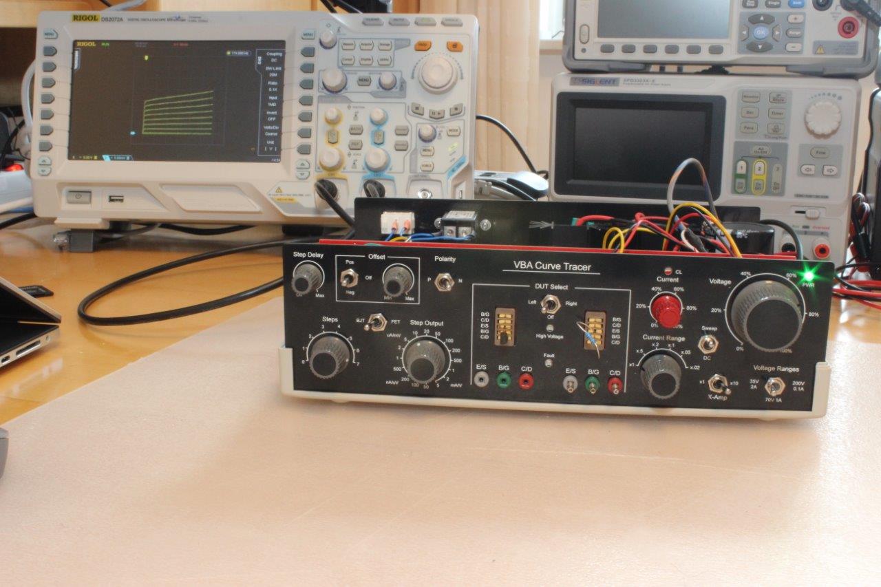
Everything here assumes the instrument as built — a fully analog sweep-and-step generator whose output is an X drive and a Y drive fed straight into an oscilloscope running in X-Y mode. There is no microcontroller, no host PC, no capture software, and no on-screen cursor readout. The scope is the display, and every number in this volume is read off the graticule with the mental arithmetic that curve tracing has always demanded. That constraint shapes how you work: you set the axes with the range controls, you set the family with the step controls, and you interpret the picture yourself.
4.1 Setting up a measurement
The controls that matter for every measurement are the same handful covered in Vol 3, and the safe order to touch them almost never changes.
Start conservative. Pick the Voltage Range that comfortably exceeds the main-terminal voltage you want to see — 35 V, 70 V, or 200 V — rather than reaching for the top range by reflex, because the higher ranges trade current headroom for volts (0–35 V at up to 2 A, 0–70 V at up to 1 A, 0–200 V at only 100 mA). Set the Current and Current Limit low. Choose a Current-range multiplier — the six settings run ×1, ×0.5, ×0.2, ×0.1, ×0.05, ×0.02 — that keeps the vertical (current) axis on-screen and the device inside its safe dissipation. Select the device type (BJT or FET) and set Polarity to N for NPN / N-channel or P for PNP / P-channel. Dial the number of Steps (0 to 7, i.e. up to eight traces counting the zero step) and a Step Output magnitude from the 1-2-5 sequence (5 V / 5 mA at the top down to 50 µV / 50 nA). Give yourself some Step Delay — the per-cycle delay is adjustable roughly 40–250 ms — whenever you are working at real power, so each trace has time to settle without cooking the part. Then bring the Voltage and Current controls up gently and watch the family grow into the screen.
The single most important habit with any curve tracer is current limiting. It is genuinely easy to destroy the device under test — the whole point of the adjustable limit and the per-step cycle delay is to stop that from happening. Set the limit before you turn anything up, not after you see smoke.
4.1.1 Getting a clean trace on the scope
Because the scope is the instrument’s only display, its X-Y performance is part of the measurement. Versteeg drove the writeup with a Rigol DSO and a few settings that carry over to any modern digital scope: use a deep record (a large sample memory, tens of thousands of points, so the swept trace is drawn from plenty of samples rather than a sparse dotted line), and apply a modest bandwidth limit (a 20 MHz limit tames broadband noise on the trace). On an analog CRT scope none of this applies — you simply run X-Y and set the gains — but the trade there is no persistence controls and no easy way to freeze a family.
One honest limit lives here: at the most sensitive current settings the trace is drawn at very small scope deflections, and DSO noise at extreme sensitivity (on the order of 100 µV/div) sets the floor on how small a leakage current or how fine a difference between two devices you can actually resolve. The tracer will happily present a µA-level detail that the scope then buries in grass.
4.2 Reading a bipolar transistor
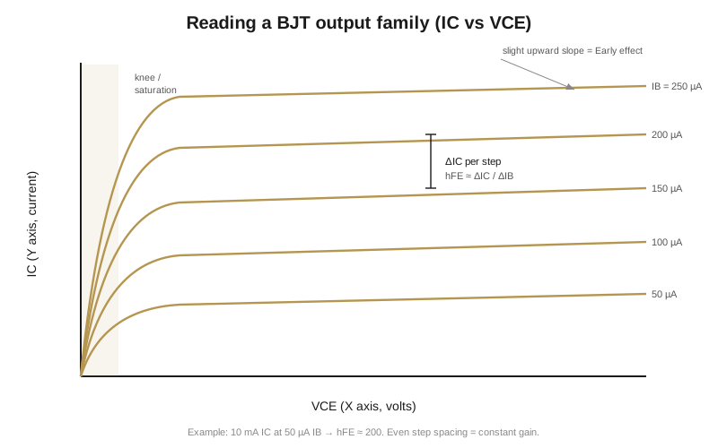
The BJT is the canonical curve-tracer subject and the one that most repays a careful read. It produces the classic fan of output curves: horizontal axis VCE, vertical axis IC, one curve per base-current step.
4.2.1 The steps and the axes
Set the step generator to base current — say 50 µA per step — and the family draws itself: the first curve is IB = 50 µA, the second 100 µA, the third 150 µA, and so on up to the seventh step. The zero step (IB = 0) sits on the baseline and is worth keeping in the family because it is where you read leakage. Set the Voltage Range so the collector sweep spans the VCE you care about, and pick a current multiplier that puts the top curve near the top of the graticule without railing it.
4.2.2 Gain (hFE / β)
Pick a curve, read its collector current off the vertical axis, and divide by that curve’s base current. As an illustration of the arithmetic, a curve sitting at IC ≈ 10 mA for IB = 50 µA gives hFE ≈ 10 mA / 50 µA = 200. The picture tells you more than the single number, though — the spacing between adjacent curves is the incremental gain. Evenly spaced traces mean constant gain across the family; traces that bunch together toward the top show gain falling off as collector current rises. That fall-off (β droop at high current) is exactly the behaviour a single hFE reading on a DMM cannot show you.
4.2.3 The knee and saturation
Down at low VCE the curves rise steeply out of the origin — the saturation region — before bending over into the flat active region. That knee is VCE(sat): it is how far above zero the collector has to be before the transistor stops behaving like a closed switch. On the VBA you can read that knee directly and lay it against the part’s datasheet VCE(sat) figure — the sort of close-but-real agreement the instrument is there to confirm.
4.2.4 The Early effect
The “flat” active region is not truly flat. It tilts gently upward — collector current creeping up as VCE increases. That slope is the Early effect; projecting the sloped lines backward to where they would cross zero current gives the Early voltage. A steeper slope means a softer device with lower output impedance, which matters if you are choosing a part for a current source or a gain stage where output impedance sets the performance.
4.2.5 Datasheet reality check
The value of seeing the whole family is that you can lay it against the datasheet’s hFE-versus-IC curve directly. The 2N3904 example lines the display up against the spread published on the 2N3904 datasheet — roughly hFE 40 minimum at 0.1 mA, 100–300 at 10 mA, 30 minimum at 100 mA — and either confirms the part is in family or flags it as an outlier or a counterfeit. This is the everyday reason to own a tracer: not to generate a number you could read off a meter, but to verify a part behaves the way its datasheet claims across its operating range.
4.2.6 Leakage currents
With the base at zero step (or specific terminals shorted/opened) the tracer reads the small reverse currents that a good part should barely show. The collector–emitter leakage with the base open is ICEO; with the base shorted to the emitter, ICES; through a resistor, ICER; the collector–base junction leakage is ICBO, and the emitter–base leakage IEBO. On the VBA these show as a faint lift of the zero-step trace off the baseline, and reading them well is where the DSO’s noise floor bites — a genuinely low-leakage part may sit right down in the scope’s grass at the sensitivity needed to see it.
4.2.7 Breakdown tests
By connecting only some of the leads you pull out the transistor’s different breakdown voltages. Base open (collector and emitter driven) gives BVCEO — a small-signal part like the 2N3904 (40 V spec) breaks down comfortably within the 70 V range. Emitter open (collector and base driven) gives the higher BVCBO; and the emitter–base junction breaks down at BVEBO, typically only a handful of volts. The higher breakdowns push you onto the 200 V range, where the 100 mA current ceiling and a tight current limit are exactly what keep the test from turning destructive. Watch for snap-back and set the limit low before you sweep.
4.3 Diodes, LEDs, Zeners and Schottky
A two-terminal part traces as a single curve rather than a family — there is no control terminal to step, so the step generator sits idle and you read the one line the sweep draws.
4.3.1 Ordinary silicon diodes
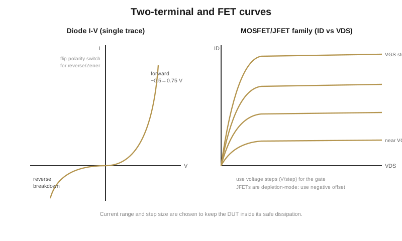
In the forward direction (anode to the swept terminal, cathode to the return) you see the conduction knee — for a silicon signal diode such as the 1N4148 it rises through the familiar exponential forward curve as current climbs, a quick health check that the junction is intact and not resistive. Flip the Polarity switch to see the reverse region, where the tracer shows the diode’s reverse breakdown against its rated minimum — real small-signal diodes routinely exceed their rated reverse voltage, and the tracer shows you by how much.
4.3.2 Schottky diodes
A Schottky such as the 1N5819 traces the same way but with a distinctly lower and softer forward knee than a silicon junction — the metal–semiconductor barrier conducts a few tenths of a volt earlier than the ~0.6–0.7 V silicon knee. Put a Schottky and an ordinary diode up on the same axes and the difference in turn-on voltage is obvious at a glance, which is the whole reason to reach for a Schottky in a low-drop rectifier or a clamp.
4.3.3 Zeners
A Zener is read in reverse, exactly like the reverse region of an ordinary diode: flip Polarity and the curve stands up sharply at the Zener voltage. What the tracer adds over a meter is the shape of that stand-up. On a 10 V Zener the reverse curve stands up near its rated voltage, and the finite tilt of the curve as current rises is the device’s dynamic (slope) resistance — the thing that decides how well it regulates. A hard, near-vertical knee is a good reference; a soft, sloped one is a mediocre one, and you can only tell them apart by looking at the curve.
4.3.4 LEDs
An LED shows a forward knee whose voltage depends on the emitted colour, because the forward voltage tracks the band-gap that sets the wavelength. A longer-wavelength red LED turns on at a lower forward voltage than a shorter-wavelength blue or white one, so their knees sit at visibly different points on the axis. That is the same physics that lets a red LED run happily from a simple resistor dropper on a low supply while a blue or white one needs noticeably more headroom — and on the tracer you read the required headroom straight off the knee.
4.4 MOSFETs and JFETs
FETs are traced as a drain-current family stepped by gate voltage rather than base current, so switch the device type to FET and set the Step Output in volts. The wrinkle with FETs is always where the interesting action sits on the gate axis, and that is what the Offset control is for.
4.4.1 Enhancement-mode MOSFETs
An enhancement MOSFET is normally off and turns on only above a positive (N-channel) or negative (P-channel) gate threshold. The useful part of the family therefore sits bunched near VGS(th), so use the Offset to slide the zero step up near the threshold and step from there rather than wasting steps down in the dead region below turn-on. A small-signal part’s threshold is typically a volt or two; Versteeg’s small-signal example is a P-channel LP0701, traced on a modest current range. Watch temperature and lean on the step-cycle delay for thermal protection, because a MOSFET in its linear region turns volts times amps straight into heat.
For a high-voltage part such as the N-channel STW6N90K5 you move onto the 200 V range to see the drain characteristic out toward its rated BVDSS, and the 100 mA ceiling of that range is what keeps the avalanche test from becoming a one-shot. The low-VDS slope of the on-curve is the device’s RDS(on) — a shallower rise means lower on-resistance — so the tracer reads switching-FET quality directly.
4.4.2 JFETs — IDSS and pinch-off
A JFET is depletion-mode: normally on. With gate and source shorted (VGS = 0) it passes its full saturation current IDSS, and you close it by driving the gate negative (for an N-channel part) until the channel pinches off at VGS(off) (equivalently VP). The transfer curve — drain current against gate voltage — is the natural way to see this: it runs from IDSS at zero gate voltage down to zero at pinch-off, following the familiar square law.
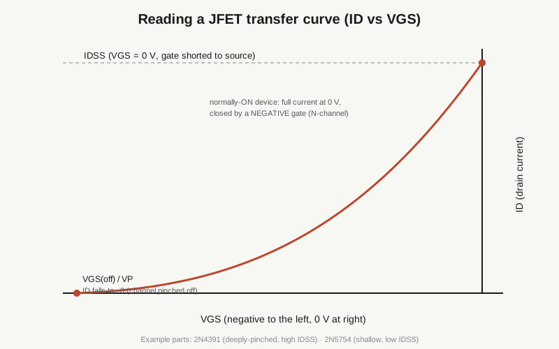
Two example parts from the measurements bracket the range you meet in practice: the 2N4391, a deeply-pinched high-IDSS part, and the 2N5754, a shallow low-IDSS part. The catch is the offset range. The standard Offset is ±2 V, which is not enough negative gate swing to reach the pinch-off of a part that closes off beyond about −5 V, as the 2N4391 does. Two ways out: fit the documented ±10 V offset modification, which extends the internal step generator’s reach to cover deeply-pinched parts, or supply external gate bias. A shallow part such as the 2N5754 pinches off well inside the standard ±2 V and needs neither.
4.5 Darlingtons and matched pairs
4.5.1 Darlingtons
A Darlington reads as a BJT family, but two junctions in series shift the numbers you expect: the effective VBE is roughly doubled (two forward drops before it conducts), the composite hFE is very large (the product of the two stages), and the VCE(sat) floor is higher than a single transistor’s because it can never fall below a diode drop. The family still fans out the same way, so the read is familiar — you just interpret the larger gain and the raised saturation floor as signatures of the compound device.
4.5.2 Matching pairs
The front panel’s DUT Select switch and its Left / Right device positions exist for exactly this. Trace one candidate, note its family, then flip to the other under identical settings and overlay the two. Parts whose families sit on top of one another — same knee, same step spacing (same hFE, or same IDSS for FETs), same active-region slope — are a matched pair. This is the everyday reason to keep a tracer on the bench when you build differential input stages, current mirrors, or complementary output pairs, and it is far more informative than matching on a single hFE number, because you are matching the whole curve across the operating range rather than agreeing at one bias point and diverging everywhere else.
4.6 Capacitor leakage
The tracer will also read the leakage of a capacitor — most usefully an electrolytic, where leakage current is a genuine health metric. Put a DC voltage across the cap (a range within its rating), let it charge, and read the small residual current that keeps flowing: a healthy cap settles to a tiny leakage, a tired or reforming one holds a stubbornly higher current. It is a slow test — the cap’s own time constant means you are watching the trace settle rather than reading an instantaneous family — and it is the one place where a long Step Delay and patience matter more than any step setting.
4.7 Limits and gotchas
- You can destroy the DUT. Curve tracing deliberately runs devices near their limits. Always set the current limit first; use Step Delay at high voltage or current to cut average dissipation and stop the curves from “blooming” (drifting as the die heats). Versteeg’s power-device examples (an MJL3281A among them) cap current explicitly — running one without a limit “could have killed the transistor.”
- Range and multiplier interactions. The current-range multipliers run ×1 down to ×0.02; pick one that keeps the family on-screen without driving the DUT supply into its current limit. With a high-power part such as the MJL3281A you step the base in small increments and cap the current for the range — push the current setting too hard and the supply simply hits its limit and the family flattens against the ceiling instead of resolving.
- The step offset is not a calibrated voltmeter. For precise gate-bias work, confirm the actual offset and step voltages with an external DMM rather than trusting the dial position.
- Deeply-pinched JFETs need more negative gate swing than the standard ±2 V offset provides. Fit the ±10 V offset modification or add external bias for parts that pinch off beyond about −5 V.
- It needs your scope, and the scope has a noise floor. The VBA has no built-in screen, so measurement quality depends on the scope’s X-Y performance and your record-length and bandwidth settings — and DSO noise at extreme sensitivity (around 100 µV/div) sets the limit on the smallest leakage currents and the finest device differences you can resolve.
- It is an analog instrument, and it is not a Tek 577. There is no data logging, no cursor readout, and no automated parameter extraction — you read values off the graticule. The envelope is bounded too: 2 A maximum caps high-current work, and 200 V maximum caps high-voltage breakdown testing — and it is nowhere near enough voltage for vacuum tubes, which is why the tube tracers (the uTracer and eTracer family) live in a separate part of the bench. Those bounds are the deliberate trade for a buildable, affordable, all-analog instrument that turns a scope you already own into a real component characteriser.
Used with a little discipline, the VBA tells you not just whether a part works, but how well — its gain across current, the shape of its knee, the tilt of its active region, where it breaks down, and whether two of them are genuinely alike. That is the whole point of a curve tracer, and this one earns its place by delivering it from four boards, a scope, and a careful hand on the current limit.