Curve Tracers — Vol 1: What a Curve Tracer Is

1.1 The one-sentence definition

A curve tracer is a test instrument that sweeps a voltage across a device, measures the current that flows, and plots current against voltage directly — turning the behavior of an active device into a picture you can read at a glance. Where a multimeter hands you a single number and a tube tester hands you a “good/weak” verdict, a curve tracer hands you the whole I-V characteristic: the map of how current responds to voltage across the device’s entire operating range.

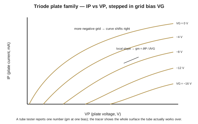
That plotted line — current on the vertical (Y) axis, voltage on the horizontal (X) axis — is the characteristic curve. For a two-terminal part like a resistor or a diode you get a single curve. For a three-terminal device like a transistor or a vacuum tube you get a whole family of curves, one per setting of the control terminal (the transistor’s base, the FET’s gate, the tube’s grid). Reading that family is the entire skill, and Vol 4 is devoted to it.

The word directly is doing real work in that definition. Any bench could, in principle, measure an I-V curve the slow way: set a supply to 1 V, write down the current; set it to 2 V, write down the current; repeat forty times; plot the column of numbers on graph paper. That is a point-by-point characterization, and it is exactly what a curve tracer automates and then does thousands of times per second. Instead of forty hand-logged points you get a continuous glowing trace, redrawn dozens of times a second, live, while your other hand is still turning the range knob. The curve tracer is not measuring anything a patient technician with a bench supply and a DMM could not measure — it is measuring all of it at once, continuously, and drawing the answer.

1.2 Why plot it — the case against the single number

Consider a bipolar transistor’s current gain, β (also written hFE), defined as the ratio of collector current to base current:

β = IC / IB

A datasheet or a component tester might tell you β = 180. That number feels solid. It is not. β is not a constant — it is a single reading pulled off a curved surface at one particular spot, and the spot is rarely where you are actually going to run the part.

Walk the surface and watch β move:

• At low collector current — say IC = 100 µA — β sags. The recombination current in the base-emitter junction is a larger fraction of the total, so gain is down. A part rated β = 180 at IC = 10 mA might deliver β ≈ 90 at 100 µA.
• In the mid-current sweet spot — a few milliamps to some tens of milliamps for a small-signal part — β peaks. This is the datasheet’s happy number.
• At high collector current — approaching the device’s power or high-injection limit — β rolls off again as the base conductivity is swamped by injected carriers.
• With collector-emitter voltage — β climbs slightly as VCE rises, because the effective base gets thinner. That tilt is the Early effect (Vol 4), and on the tracer it shows up as the family of output curves sloping gently upward instead of running dead flat.
• With temperature — β typically rises on the order of +0.5 % to +1 %/°C for silicon, so a part that self-heats under test reads higher gain hot than cold.

A single number is a single point sampled off a surface that is anything but flat. The curve tracer shows you the shape of that surface, so you can see where β is flat enough to trust, where the device saturates, where it breaks down, and — the classic use — whether two “matched” parts really track each other or merely happen to agree at the one bias point where somebody measured them.

That last point is worth dwelling on, because it is where the picture earns its keep on a working bench. Two transistors that both read β = 180 on a component tester can have curve families that diverge badly at the edges: one holds gain down to 100 µA and the other collapses; one breaks down at 60 V and the other at 45 V. For a differential pair, a push-pull output stage, or a current mirror, it is the agreement across the whole surface that matters, not agreement at one arbitrary point. You cannot see that with a number. You can see it in a heartbeat by overlaying two curve families on the same screen — matched parts lie on top of each other; mismatched parts fan apart, and exactly where they fan apart tells you where the circuit built from them will misbehave.

This is the recurring theme of the whole instrument class: an active device is a surface, not a number, and the curve tracer draws the surface. Once you have seen a leaky transistor’s family of curves refuse to close down to zero at IB = 0, or watched a tired vacuum tube’s plate curves sag below the datasheet grid, you stop trusting single-point measurements for anything that matters.

1.3 What the picture actually contains

Before we build the instrument, it is worth naming what shows up on the screen, because every feature is a device parameter you would otherwise have to hunt for one probe at a time. Vol 4 teaches you to read these quantitatively; here is the vocabulary so the rest of the primer has words to use.

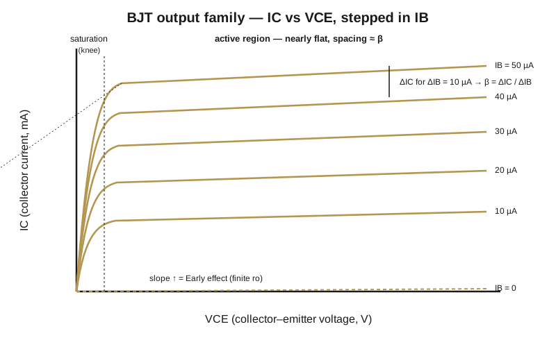
The knee. Down near the origin every output curve rises steeply out of zero before bending over. That steep rise is the saturation (or ohmic) region, where the device looks like a small resistance; the bend is the knee. On a transistor the knee marks VCE(sat) — a few tenths of a volt — the floor below which the part can no longer regulate current. On a power MOSFET the slope of that rising region is RDS(on), the on-resistance you care about in a switching supply.

The flat. Past the knee the curve runs nearly horizontal — the active region for a BJT, saturation for a FET (the naming is unfortunately reversed between the two device types). Here the device behaves as a controlled current source: change the terminal voltage and the current barely moves. How horizontal the flat runs, and how evenly the flats are stacked, is what you buy a curve tracer to see.

The spacing. The vertical gap between adjacent curves in the family is the device’s gain. For a BJT stepped in base current, equal steps of IB that produce equal gaps of IC mean constant β; gaps that widen or pinch as you climb the family are β varying with current, drawn to scale. For a FET or a tube stepped in voltage, the spacing is the transconductance, gm = ∂Iout/∂Vin, measured in siemens (or the old mhos and µmhos on tube data).

The slope of the flat. Not perfectly flat — the gentle upward tilt is output conductance, the finite output resistance ro. Extrapolate the flats leftward and, for a BJT, they converge on a single point on the negative voltage axis: the Early voltage, VA. A steep tilt means low ro and a poor current source.

The breakdown wall. Push the sweep voltage high enough and every curve turns and shoots vertically upward — current running away at nearly constant voltage. That wall is the breakdown voltage: BVCEO for a transistor, the avalanche or zener point for a diode. The tracer draws it as a hard corner, and its current-limit resistors are what keep the device alive long enough for you to read the voltage off the screen instead of vaporizing the part.

Leakage and lifelessness. With the control terminal at zero, a healthy part sits on the baseline — the IB = 0 curve hugs the voltage axis. A curve that floats above the axis at zero drive is leakage; a whole family crammed together with almost no spacing is a dead or gainless device. Both are diagnoses you make at a glance and would struggle to make with a meter.

1.4 The two big families of curve tracer

Curve tracers split into two lineages by what they are built to test. The physics of drawing an I-V curve is identical; the voltage levels, the safety envelope, and the fixturing are wildly different.

Semiconductor curve tracers test transistors, diodes, FETs, SCRs, and other solid-state parts. This is the classic transistor-lab instrument — the Tektronix 575/576/577 lineage (Vol 2), the Heathkit IT-1121/IT-3121 hobby units, and modern DIY designs. They step the control terminal in small increments — microamps of base current, or a volt or two of gate voltage — and sweep the main terminal from zero over a range that runs from a few volts up to, on the big vintage iron, well over a kilovolt. The two specific instrument dives in this hub on this side of the line are the Heathkit IT-3121 (a vintage analog unit that drives an external scope in X-Y; collector to ±200 V, current to 1 A) and the VBA Curve Tracer (a fully analog open-source design named for its authors Versteeg, Bennett, and Allie).

Tube curve tracers test vacuum valves. A triode or pentode wants hundreds of volts on its plate and a screen, and its “control terminal” is a negative grid bias rather than a forward base current. The archetype is the Tektronix Type 570 (1955, Vol 2), and the modern revival is a set of pulsed-HV designs that charge a reservoir capacitor and fire the tube for roughly a millisecond so the average dissipation — and therefore the heat, the power supply, and the danger — stays manageable. Three of them are dives in this hub: the eTracer (a commercial USB tube tracer from Essues in Taiwan, anode 0–750 V — not a Dekker design), the uTracer6 (Ronald Dekker’s kilovolt DIY model, 0–1000 V, reaching sweep and transmitter tubes), and the uTracer NXT (Dekker’s next-generation DIY design, 450–500 V, the current mainstream). Their pulsed-HV method is the subject of Vol 3.

A useful way to hold the distinction: the semiconductor tracer steps a current into the base; the tube tracer steps a voltage on the grid. Both then sweep the main-terminal voltage and plot the resulting current. The rest of the difference is mostly the size of the voltages and how carefully you have to respect them — a bench transistor tracer at 20 V is casual, a tube plate sweep at several hundred volts is not.

One naming trap worth flagging now and settling in Vol 2: the Tektronix 575, the first transistor curve tracer (March 1957), is itself built from vacuum tubes. It is a tube-based instrument for testing transistors. “Tube tracer” and “semiconductor tracer” describe what the instrument is for, not what it is made of.

1.5 The block diagram — three parts and a plot

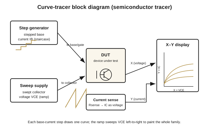
Nearly every curve tracer, from a 1957 Tektronix to a modern DIY board, is built from the same three functional blocks. Learn them once and you can read any tracer’s front panel, tube or semiconductor, vintage or new.

1.5.1 The step generator

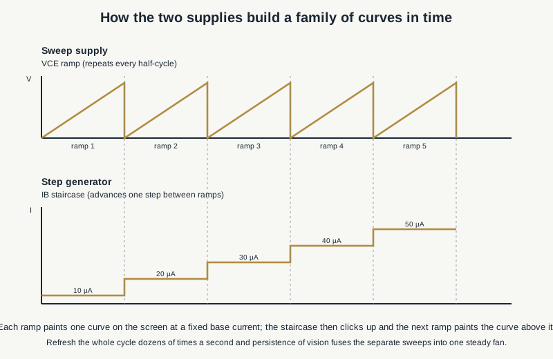
The step generator drives the control terminal. In a semiconductor tracer it produces a staircase — a series of equal current (or voltage) steps, one per curve in the family. Set it to 10 µA/step with 5 steps and the instrument draws five curves at base currents of 10, 20, 30, 40, and 50 µA. Set it to 0.2 V/step for a MOSFET gate and it draws curves at 0.2, 0.4, 0.6 V, and so on. The step generator is what turns a single I-V curve into a family; without it you would trace one curve at a time and re-set the bias by hand between each.

Two controls on this block matter constantly: the step size (amps or volts per step) sets the vertical scale of the family, and the number of steps sets how many curves you draw. Push the step size too large and the top curve drives the device past its power limit; too small and the whole family collapses into one fat line. In a tube tracer the same block generates stepped negative grid voltages instead of stepped base currents — the grid is normally biased below the cathode, and the staircase walks it from, say, −16 V toward 0 V in a handful of steps.

1.5.2 The sweep supply

The sweep supply — called the collector supply on a semiconductor tracer, the plate supply on a tube tracer — drives the main terminal. It ramps the voltage from zero up to a selectable maximum and back, over and over. Each sweep paints one curve left-to-right across the screen; the staircase advances one step between sweeps, so the beam paints the next curve up. Do this fast enough and persistence of vision fuses the separate sweeps into a steady family of curves.

Classic analog tracers take a clever shortcut here: the sweep supply is just rectified line voltage. A variable transformer feeds a rectifier, and each half-cycle of the AC mains is one voltage ramp — 0 up to peak and back to 0 in 8.3 ms on a 60 Hz line. The step generator is clocked off the same mains, advancing one step every half-cycle (or every full cycle). That is why the collector supply on a vintage Tek is specified as peak volts and reads as a raw rectified sine, and why the family refreshes at line rate. It is elegant: the mains does the ramping for free, and synchronizing the staircase to it is trivial.

The single most important thing to understand about the sweep supply is that its maximum voltage and its maximum current live on different range positions. A curve tracer’s range switch does not offer “1500 V and 20 A at once” — it offers 15 V at 10 A on one position, and 1500 V at 0.1 A on another, with a fixed series resistor sizing each. On the Tektronix 576 (1969) the four collector ranges are 15 V/10 A, 75 V/2 A, 350 V/0.5 A, and 1500 V/0.1 A; the highest voltage is available only at the lowest current, and vice versa. So when the vintage iron is described as reaching “~1.5 kV,” that is a range ceiling, not a simultaneous V × I capability. The series resistor that lets you put 1500 V across a device is exactly the resistor that limits the current to 0.1 A, and it is there to keep both the device and the operator alive. The Tektronix 577 (November 1972) sits alongside the 576 with a similar story — its top sweep range reaches 1600 V at 40 mA — and the two were contemporaries, not a strict succession, before both gave way to the digital 370-series. (The full lineage and its verified dates are Vol 2’s job.)

1.5.3 The X-Y display

The X-Y display plots the result. The main-terminal voltage drives the horizontal axis; the sensed current drives the vertical axis. There is no time base — the horizontal position is voltage, exactly as in an oscilloscope’s X-Y mode. The beam does not sweep left-to-right on a clock; it goes wherever the device’s operating point currently sits, and because the sweep supply is dragging the voltage from 0 to peak, the operating point traces out the curve as a natural consequence.

How the display is realized is one of the clearest dividing lines between generations of tracer:

• Vintage integrated CRT. The Tektronix 570/575/576/577 each carry their own calibrated CRT with a graticule marked directly in volts-per-division and current-per-division. You read the curve off the tube like a scope.
• Bring-your-own scope. The Heathkit IT-3121 and many DIY analog designs — the VBA Curve Tracer among them — have no display of their own. They output an X (voltage) signal and a Y (current) signal and expect you to put your bench oscilloscope in X-Y mode. Cheaper to build; you already own the scope.
• Digitize and plot in software. The pulsed-HV tube tracers — the eTracer, the uTracer6, and the uTracer NXT — take single-point measurements, sample the voltage and current at each pulse, stream the numbers to a PC over USB, and let host software draw the curves. The “display” is a window on your laptop, the curves are stored data you can export, and (on the eTracer, for instance) the software can even fit a SPICE model to what it measured.

1.5.4 The current-sense element

Between the sweep supply and the display sits a current-sense element — usually a small, precise resistor in the return leg of the device. The device current flows through it and develops a proportional voltage (Ohm’s law, V = I·Rsense) that the Y channel of the display can plot. Pick Rsense = 1 Ω and 100 mA of collector current becomes 100 mV on the Y axis; switch to a 100 Ω sense resistor and 1 mA becomes the same 100 mV — that range-switching of the sense element is what gives the vertical axis its selectable amps-per-division. In the digitizing DIY tracers the same job is done by a sense resistor feeding an amplifier and an ADC, but the principle is identical: current is measured as the voltage across a known resistance.

Everything else on the front panel — the dissipation-limiting series resistors, the collector-supply range switch, the polarity-reversal switch that flips the whole picture for NPN versus PNP (or N-channel versus P-channel), the step-family controls — is there to keep the device safe and to scale the picture. Vol 3 walks through each control in turn.

1.6 What you are looking at, in one glance

Put those three blocks together and here is what happens each cycle. The step generator sets the base to, say, 20 µA and holds it. The sweep supply ramps VCE from 0 up to 20 V and back. The sense resistor reports the collector current at every instant along the way. The display draws a curve rising steeply from the origin, bending over at the knee near a few tenths of a volt, then running nearly flat across the screen at whatever IC that 20 µA of base drive commands — for β ≈ 150 that flat sits around IC = 3 mA. The staircase clicks to 30 µA and the next ramp draws a higher curve, its flat now near 4.5 mA. Five or ten steps later you are looking at a fan of curves — the transistor’s output characteristics — refreshed dozens of times a second, steady and live, every feature from the previous section visible at once.

Turn the collector-supply knob and the curves stretch or compress horizontally as the voltage range changes. Turn the step size and the fan opens or closes vertically. Flip the polarity switch and the whole picture mirrors into the opposite quadrant for the complementary part. Nothing here is subtle once you have the three blocks in your head: a staircase into the control terminal, a ramp into the main terminal, a sense resistor turning current into a Y voltage, and an X-Y screen tying it together.

1.7 The simplest curve tracer of all — the octopus

You do not need any of that machinery to draw an I-V curve. Strip the instrument down to its irreducible core and you get the “octopus” — the poor technician’s curve tracer, and the fastest way to internalize what a curve tracer is.

The entire circuit is a filament transformer and a resistor. A small transformer — the 6.3 V heater winding out of a dead tube radio is the traditional choice — drops the mains to a low AC voltage. That AC is fed through a current-limiting resistor to the unknown component. Then you wire two signals to an oscilloscope running in X-Y mode: the voltage across the device goes to X (horizontal), and the voltage across the series resistor — which is proportional to the current through the device — goes to Y (vertical). That is it. No step generator, no sweeping ramp, no calibrated CRT of its own. The AC line does the “sweeping” — every mains cycle drives the device from a positive peak, through zero, to a negative peak and back, so the operating point walks up and down the device’s I-V curve fifty or sixty times a second, and the scope draws the loop.

Because the drive is AC and covers both polarities, the octopus draws the device’s signature in all four quadrants at once, and each class of part traces a distinctive shape — a Lissajous signature:

• Open circuit — no current can flow, so Y stays at zero: a flat horizontal line.
• Short circuit — no voltage can develop, so X stays at zero: a vertical line.
• Resistor — current is proportional to voltage (Ohm’s law), so the trace is a straight sloped line through the origin; the steeper the slope, the lower the resistance.
• Capacitor — current leads voltage by 90°, so X and Y are in quadrature and the trace opens into an ellipse; a fatter ellipse means more capacitance at that test frequency.
• Inductor — current lags voltage, again drawing an ellipse (tilted the other way), usually with series-resistance flattening it toward a slanted line.
• Diode — conducts one way and blocks the other, drawing a backward-L / knee shape: a flat leg while blocked, a sharp corner at the forward voltage, then a steep leg while conducting.
• Transistor junction — read one junction at a time, it shows a diode knee forward and, if driven hard enough, a reverse-breakdown corner.

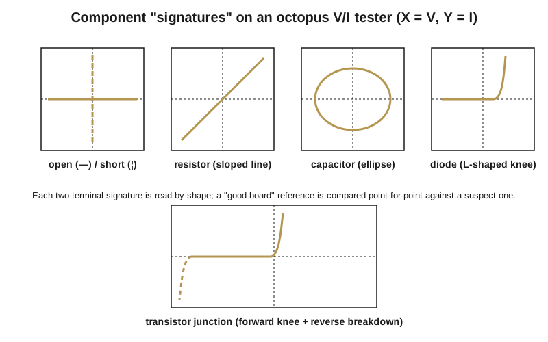
This same technique, dressed up with a reference board and standardized test levels — typically around 1 V open-circuit and under a milliamp of current, gentle enough to probe a live-looking node without turning anything on — is sold commercially as Analog Signature Analysis (ASA), and it is a mainstay of no-power board troubleshooting: you compare the signature at a node on a suspect board against the signature at the same node on a known-good board, point for point, and any component that has drifted, shorted, or opened shows up as a signature that no longer matches. The name “octopus” comes from the tangle of test leads sprouting off the box.

The octopus is worth building — an evening’s work from a junk-box transformer, one resistor, and a scope — precisely because it makes the definition physical. Sweep a voltage (the AC line does it), measure the current (the series resistor does it), plot one against the other (the scope in X-Y does it). Everything else in this primer is that same idea with more voltage, a controlled staircase into a third terminal, and better instrumentation wrapped around it. The octopus and its scope-adapter cousins get their full treatment, alongside the real instruments, in Vol 5.

1.8 Where this goes next

Everything in the rest of this primer builds on the picture you now have — three blocks, a sense resistor, an X-Y screen, and the octopus as the stripped-down proof of the idea.

• Vol 2 traces where the instrument came from: the Tektronix lineage with its verified dates — the tube-oriented Type 570 (1955), the first transistor tracer Type 575 (March 1957, and itself a tube instrument), the mature analog 576 (1969, to 1500 V) and 577 (November 1972, to 1600 V at 40 mA) as contemporaries, and the digital GPIB-programmable 370/370A (1986, ±2000 V / ±20 A) — plus the tube-tester-versus-curve-tracer distinction and the modern DIY revival.
• Vol 3 explains how each type actually generates the sweep and what every control does — the stepped-base/swept-collector semiconductor tracer, the charge-a-cap-and-pulse tube tracer of the uTracer and eTracer dives, and the octopus.
• Vol 4 teaches you to read the fan of curves quantitatively — β from curve spacing, transconductance and gm, the Early effect, breakdown, the saturation knee, and device matching — along with the traps: parallax, range ceilings, and thermal drift.
• Vol 5 lays out today’s buy-versus-build landscape — the vintage Tek iron, the Heathkit IT-3121, the scope-adapter and octopus approaches, and the modern DIY designs (the eTracer, uTracer6, uTracer NXT, and VBA Curve Tracer) — and points you at which to reach for.