Curve Tracers — Vol 3: How They Work

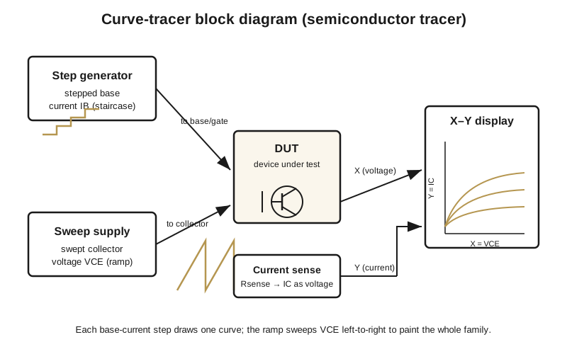
Vol 1 gave you the three blocks — step generator, sweep supply, X-Y display — and the reason they exist: a single number tells you almost nothing about an active device, but the shape of its current-vs-voltage family tells you nearly everything. This volume opens each of the three main kinds of tracer to show how those blocks are actually built in copper and silicon (and, for the tube tracers, in a charged capacitor), then walks the standard front-panel controls so you can sit down cold at any tracer and know what each knob is doing to the device on the fixture.

Three families cover the whole landscape. The semiconductor tracer — stepped base/gate and a swept collector, painting a live family on a CRT or your own scope — is the Tektronix 575/576/577 and the Heathkit IT-3121, and it is the one to understand first because the other two are variations on the same idea. The pulsed-HV tube tracer solves the same measurement for a device that wants hundreds of volts by charging a capacitor and firing it at the tube for about a millisecond; that is the uTracer6, the uTracer NXT, and the eTracer. The octopus throws away the step generator entirely and reads two-terminal devices by the Lissajous shape they draw. Get these three, and every instrument in this hub is a point on the same map.

3.1 The semiconductor curve tracer: stepped base current, swept collector

This is the architecture of the Tektronix 575 (March 1957), the 576 (1969), the 577 (November 1972), and the Heathkit IT-3121, and it is worth internalizing before anything else. Two things happen at once, locked in step: a voltage is swept across the device’s output terminals many times a second, while a control-terminal drive is advanced one notch between sweeps. The swept axis paints one curve; the stepped drive stacks the curves into a fan.

3.1.1 The collector sweep is a rectified-AC ramp, not a DC rail

The first surprise for anyone expecting a regulated bench supply: in the classic designs the collector supply produces a rectified-AC ramp, not a steady DC voltage. The mains sine wave is stepped by a transformer and rectified into a train of half-sine humps; each hump drives the collector-emitter voltage VCE from zero up to the peak set by the front-panel control and back down to zero. On a full-wave rectified 60 Hz line that is 120 humps per second — 120 complete left-to-right sweeps of the display every second, which is exactly the refresh rate you want for a flicker-free, live picture that responds the instant you turn a knob or swap a device.

There are three good reasons the classic instruments do it this way rather than regulating a DC rail and sawtoothing it electronically:

• Free synchronization. Because the sweep is derived from the same line the display timebase can lock to, every sweep starts at the same phase and the curves overlay perfectly. No trigger circuit, no timebase oscillator — the wall socket is the clock.
• Duty cycle protects the device. The device sees its full VCE only at the crest of each hump; for most of every cycle it is at low voltage or off. A transistor being pushed to its power limit is therefore dissipating far less average power than the instantaneous VCE × IC at the peak would suggest, which lets the instrument probe closer to the edge of the safe operating area without cooking the part on contact.
• It is cheap and rugged. A transformer and a bridge are a lot less to go wrong than a fast, high-compliance regulated supply — and the current the tracer can source on a peak is limited naturally by the transformer and the series resistor rather than by an active fold-back loop.

The Heathkit IT-3121 is a clean, small example of the whole scheme. Its collector supply is deliberately pulsating DC from a transformer and diodes — no expensive regulated HV rail — and a simple three-transistor Darlington buffer varies the peak from 0 up through a low and a high (~200 V) range depending on the range switch, into a collector current up to about 1 A. It drives an external oscilloscope in X-Y rather than carrying its own CRT, so the whole box is a sweep, a step generator, a current sense, and the buffers to run them. That is the semiconductor tracer stripped to its studs.

3.1.2 The base staircase steps between sweeps

Synchronized to that sweep, the step generator advances the base drive by one increment between humps — during the brief zero-crossing when the collector voltage is at the bottom of its swing and no curve is being painted. The mechanism is a small digital-to-analog staircase: a counter (a single TTL counter in the IT-3121) is clocked once per sweep, its count drives a small DAC, and the DAC output feeds a precision current source that turns each equal voltage step into an equal base-current step. Set the front panel to 5 steps and the generator dwells at 0, then 1, then 2, 3, 4, 5 increments of base current — one value held for the duration of one collector sweep, then clocked up during the next zero-crossing, and rolled back to zero to start the family again.

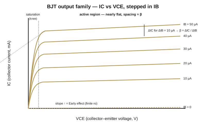
The result is Vol 1’s fan, built one curve at a time faster than the eye can follow. The beam paints the whole IC-vs-VCE curve for IB = 10 µA; the staircase clicks up; the beam paints the IB = 20 µA curve sitting above it; and so on up the family, refreshing 120 times a second so the stack looks solid and static. The IT-3121 offers step sizes ranging from microamp-scale steps for small-signal parts up to milliamp-scale steps for power devices — small enough to resolve a small-signal transistor’s base fan, coarse enough to walk a power device up to an amp of collector current in a handful of steps. Throw the polarity switches and the identical machine tests PNP devices, with the whole family reflected into the opposite quadrant of the screen.

3.1.3 Base current for a BJT, gate voltage for a FET

A subtle but load-bearing point: the right control variable depends on the device, and a good tracer switches between two behaviors for its step generator.

For a bipolar junction transistor the natural handle is base current — collector current is set by base current through the transistor’s current gain, so the step generator is configured as a current source and each curve is labelled with an IB value in microamps or milliamps.

For a field-effect transistor — a JFET or a MOSFET — the gate draws essentially no DC current; the device is controlled by the voltage on its gate. So the step generator is switched to produce equal voltage steps, and each curve in the family is labelled with a VGS value in volts. A tracer that can do both — like the VBA Curve Tracer, whose step generator can be set to stepped current or stepped voltage — characterizes BJTs, JFETs, MOSFETs, and Darlingtons from the same front panel without rewiring. When you sit down at an unfamiliar tracer, the first thing to confirm is whether the step knob is handing the device milliamps or volts, because the whole reading of the fan depends on it (Vol 4 turns those step values into β and gm).

3.2 The pulsed-HV tube tracer: charge a cap, fire it, sample once

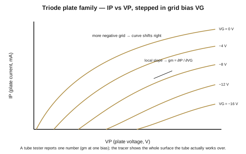
A vacuum tube wants a completely different set of conditions from a transistor: hundreds of volts on the plate, often a separate screen supply for pentodes and tetrodes, a negative grid bias as the control terminal, and a heater to bring the cathode up to emission. Tektronix’s Type 570 (1955) — the instrument that started the whole category — did this the direct way, with real high-voltage supplies and a genuinely swept plate voltage, which is exactly why it is a large, heavy, mains-hungry box. Sweeping several hundred continuous volts through a power tube means the instrument has to be able to source and dissipate serious power all day.

The modern DIY tube tracers get the same measurement out of a palm-sized board by refusing to do it continuously. This is the single cleverest idea in the category, and it is worth stating plainly: you do not need to hold the plate voltage on the tube — you only need it on the tube at the instant you take the reading.

3.2.1 The reservoir-and-pulse trick

Ronald Dekker’s uTracer designs — and the commercial eTracer that followed the same principle — charge a large reservoir capacitor up to the desired plate (and, separately, screen) voltage from a compact boost converter. Charging is slow and gentle: the little converter trickles energy into the cap over tens of milliseconds, drawing modest average current from a small DC input. Then, with the cap sitting at (say) 300 V, the instrument connects it to the tube through a fast switch for a short pulse — on the order of one millisecond — and, during that pulse, samples the plate voltage and the plate and screen currents. The switch opens, the residual charge is dumped, the grid bias is stepped to the next value, the cap is recharged, and the whole cycle repeats to build the next point in the family.

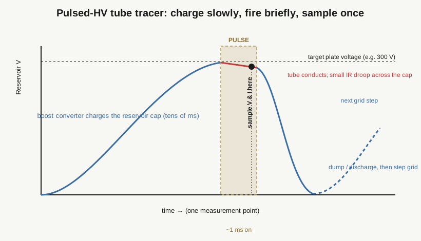
The payoff is a power ratio. Suppose you are pulling a plate point at 300 V and 50 mA — that is 15 W of instantaneous plate power, real power-tube conditions. If the pulse is 1 ms long and the instrument only fires a few of them per second, the duty cycle is a fraction of a percent, and the average power the little board has to move is milliwatts. A 1 ms conduction out of, say, a 100 ms cycle is a 1% duty cycle — 15 W instantaneous becomes 0.15 W average — and in practice the cycle is often longer and the average lower still. That is the entire reason a several-hundred-volt tube characterizer fits on a board you can hold in one hand: it never dissipates the full plate power, it only sources it for a pulse, out of a capacitor that was charged slowly.

There is a second, quieter payoff: the pulse protects the tube. A shorted, gassy, or over-driven valve conducts for a single millisecond and is then disconnected, instead of sitting there arcing or running away. The same brevity is what lets the instrument sweep a whole family safely — it steps the grid bias and re-fires the plate pulse at each grid setting, and if any one point looks wrong the damage window was a millisecond wide.

Because there is no continuous swept ramp to paint a CRT, these instruments digitize each sampled point and hand the family to host software on a PC, which draws the curves, applies calibration, and often exports a SPICE model. The takeaway for this volume: pulsed HV means big voltages, tiny average power, and host-side plotting — a fundamentally different architecture from the continuous-sweep semiconductor tracers above, arriving at the same picture.

3.2.2 The three tube tracers in this hub, and their envelopes

The per-instrument dives go into the reservoir sizing, the current-sense front ends, and the safety interlocks in detail; here is where each sits so the cross-references are unambiguous:

• The uTracer6 dive covers Dekker’s kilovolt-class DIY model, reaching 0–1000 V on the plate — enough to characterize sweep tubes, beam-power tubes, and small transmitter tubes that the lower-voltage designs cannot reach. It is a distinct high-voltage model, not a revision of the earlier uTracer3.
• The uTracer NXT dive covers Dekker’s current-generation DIY design (a new architecture, in the 450–500 V plate class), the mainstream choice for ordinary receiving tubes.
• The eTracer dive covers the commercial Essues (Taiwan) instrument — an independent design inspired by the uTracer principle rather than a Dekker product — reaching 0–750 V on the plate. It is the reach-for-it-and-go option in this hub, kit plus software rather than a from-scratch build.

All three apply genuinely lethal voltages and store real energy in that reservoir capacitor — a charged 300 V cap does not care that the instrument is small. They demand the same high-voltage bench discipline as any tube gear: this project’s shared bench-safety notes apply in full, and the reservoir cap must be treated as live until it is proven discharged.

3.3 The simple case: the “octopus” component / signature tester

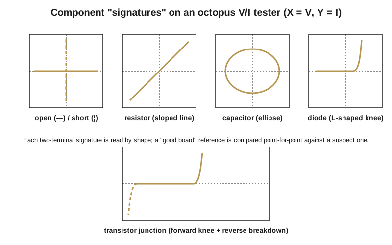
At the opposite end of the complexity range sits the octopus — the poor man’s curve tracer, so called because a shop-built one tends to sprout test leads like tentacles. It has no step generator, no counter, no swept high voltage, and often no active parts at all. It applies a small AC excitation — typically about 1 V (sometimes a few volts) at line frequency, current-limited to well under a milliamp by a series resistor — across a two-terminal device. The voltage across the device goes to the scope’s X input; the current, sampled as the voltage across the series resistor, goes to the Y input; and the scope in X-Y mode draws the resulting Lissajous “signature.” A filament transformer and two resistors is a complete octopus.

You read an octopus by shape, not by number. A resistor traces a straight sloped line whose angle encodes its value — steeper is lower resistance, because more current flows for the same voltage. A capacitor or inductor traces an ellipse, because the current leads or lags the voltage and the X-Y plot of two phase-shifted sinusoids is an ellipse; the fatter the ellipse, the more reactive the part. A good junction traces an L-shaped knee — flat while reverse-biased and below the forward turn-on, then rising sharply past ~0.6 V. An open reads as a flat horizontal line (voltage but no current), a dead short as a vertical one (current but no voltage).

Its killer feature is in-circuit testing. Because the octopus only wiggles a volt or so at sub-milliamp current, you can probe a component — or a whole node — without desoldering it and with the board unpowered, and compare a suspect board point-for-point against a known-good reference. That technique has a name, analog signature analysis (ASA), and it is how you find a leaky junction, a shorted tantalum, or an open trace on a dead board in minutes without pulling parts. What it will not give you is β, gm, or any of the three-terminal parameters Vol 4 is about — it has no control terminal to step. The octopus and the semiconductor tracer are not competitors; they answer different questions, and a well-equipped bench keeps both within reach.

3.4 What the standard controls do

Sit down at almost any semiconductor curve tracer — vintage Tek iron, a Heathkit IT-3121, or a DIY design driving your own scope — and the front panel falls into the same four clusters. Knowing what each cluster does to the device is most of the battle; the specific labels and ranges change, the functions do not.

3.4.1 The step / base controls set up the family

These decide how many curves you get and how far apart they sit:

• Steps per family — how many curves in the fan, typically selectable from a couple up to about 10. Fewer steps make a specific parameter easier to read cleanly; more steps give a denser picture of how the device behaves across its control range.
• Step amplitude — the size of each increment: microamps or milliamps per step for a BJT (current steps), volts per step for a FET (voltage steps). This sets the vertical spacing of the fan, and it is the number you divide by in Vol 4 to get gain.
• Step polarity / offset — which quadrant the family lands in (NPN vs PNP, N- vs P-channel), and, on tracers that provide it, a DC offset so you can start the step family above a threshold — indispensable for a MOSFET, whose curves do nothing until VGS climbs past its gate threshold voltage.

3.4.2 The collector / sweep controls set the horizontal extent and the power

These set how far right the ramp reaches and, with the series resistor, how hard the device is driven:

• Peak sweep voltage — the maximum VCE (or VDS) the ramp reaches at the crest of each hump; this is the right-hand edge of the picture.
• Voltage range — a coarse multiplier on the sweep (the IT-3121’s low vs ~200 V ranges are the textbook example). On the big vintage Tek machines this is where the ~1.5 kV headline lives — and it is critical to read it correctly. The 576 tops out at 1500 V and the 577 at 1600 V, but those ceilings sit on the high-voltage, low-current range positions only. Maximum voltage and maximum current live on different range-switch settings: you get 1500 V at 0.1 A on one range, or 15 V at 10 A on another, never the two extremes at once. The kilovolt figure is a range ceiling, not a simultaneous voltage-times-current capability, and reading it as the latter is how people talk themselves into expecting power the instrument was never built to deliver.
• Polarity — flips the whole sweep and step polarity together to move from NPN/N-channel to PNP/P-channel devices.

3.4.3 The series / load resistor is the one that keeps you from vaporizing the device

Often labelled series resistance, load, limit, or max peak power, this control inserts a resistor in series with the collector sweep, and it does two jobs at once. First, it limits the peak current — and therefore the peak dissipation — the device can be driven to, so a dead short on the fixture draws a finite, survivable current instead of dumping the supply into the part. Second, it sets the load line the device is tested against, which is the diagonal you read saturation and operating point against in Vol 4.

This is the control that protects the device under test, and the discipline never changes: start with high series resistance and low peak voltage, then open the throttle only as far as the measurement needs. Bringing up an unknown or expensive part on a low series-resistance, high-voltage setting is how you turn a device you were trying to characterize into an open one. On the pulsed-HV tube tracers the equivalent guard is the pulse itself plus a current-limit setting; the mindset is identical — bound the worst case before you apply it.

3.4.4 The display / scaling controls set what the picture means

A curve is a shape until you attach numbers to its axes, and that is what these do:

• Vertical (current) sensitivity — amps or milliamps per division on the Y axis.
• Horizontal (voltage) sensitivity — volts per division on the X axis.
• On instruments that plot to your own scope — the IT-3121, the VBA Curve Tracer, the DIY rigs — the corresponding V/div you dial into the oscilloscope’s X and Y channels, plus the value of the current-sense resistor, together define the scale.

On the vintage Tek machines an on-screen alphanumeric readout printed these scale factors right on the graticule, so the picture carried its own units. On a Heathkit-plus-scope or a DIY-plus-scope rig, you are responsible for tracking them, because the same fan of curves means 2 mA per division or 200 mA per division depending only on knobs you set — and a family of curves you cannot put numbers on is a pretty picture, not a measurement.

With the architecture and the controls in hand, Vol 4 turns to the actual skill the whole instrument exists for: reading the family of curves it draws — pulling β and gm off the spacing of the fan, spotting the Early effect in its upward tilt, finding breakdown and the saturation knee, and using the tracer to match devices into pairs — along with the traps (parallax, range ceilings, thermal drift) that catch people who trust the picture too far.