eTracer — Vol 3: Hardware Architecture & How It Measures

3.1 The measuring problem the hardware exists to solve

A vacuum tube’s published curves are drawn well past the plate dissipation it can survive continuously. A 12AX7 plotted to 400 V on the plate at tens of milliamps, or an output pentode plotted into its knee at several hundred volts, would dissipate far more than the envelope can shed as heat if you held that operating point with a bench supply. The classic answer was a lot of iron: a big continuous HV supply, a large series pass element, and a tube that you accept will run hot for the duration of the sweep. That is how the vintage Tek 570-class tube tracers did it, and it is why they weigh what they weigh.

The eTracer takes the other route, the same concept the uTracer popularized (Vol 2 covers that lineage and why the eTracer is an independent Essues/Chris Chang design, not a Dekker product): don’t hold the operating point at all. Charge a capacitor up to the target plate voltage, dump it onto the tube for a brief measurement pulse while you sample the plate current, then disconnect and let the tube cool. Essues calls it the flash-camera trick — the reservoir cap is the flash capacitor, storing energy slowly and releasing it in a short burst. Because the tube only sees high voltage during the pulse (500 µs to 5 ms in the eTracer), its average dissipation stays low even though the instantaneous operating point is well above its continuous rating. That is the whole reason a board roughly 21 cm × 15 cm can characterize tubes that used to demand a bench full of supplies.

This volume walks the hardware that implements that: the two HV rails, the charge/pulse/sample engine, the low-voltage supplies that set up the tube, and the converter chain that turns a pulse into a data point. Operating the resulting instrument — the host software, the scan modes, reading the curves — is Vol 4; chassis integration, calibration, and the safety discipline the stored energy demands are Vol 5.

3.2 System block diagram

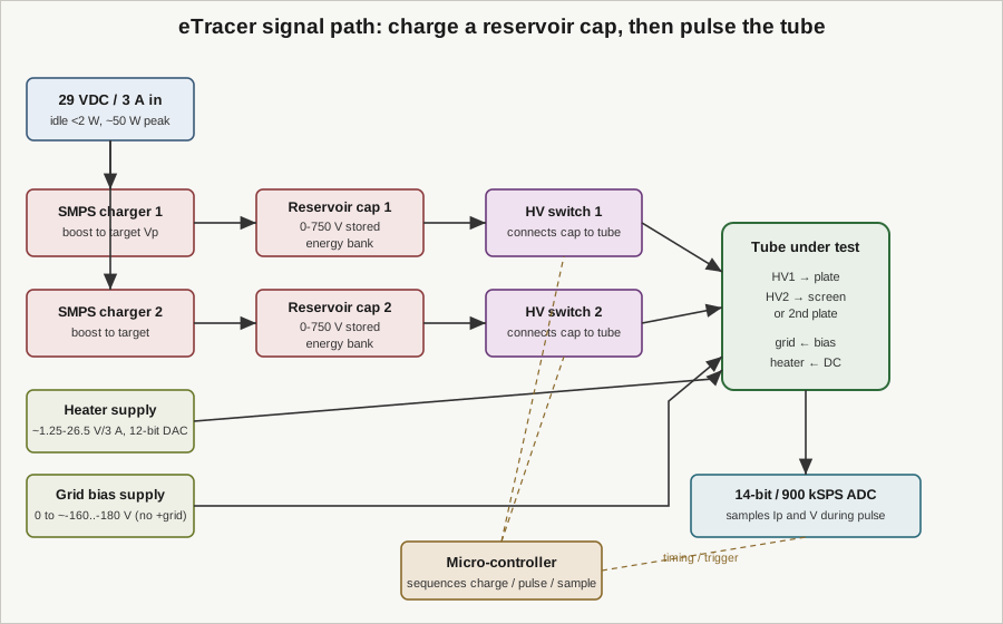
The board is a charge-and-fire engine wrapped in low-voltage support and instrumentation:

• Two identical high-voltage rails. Each is an SMPS boost converter that charges a reservoir capacitor, plus a high-side switch that connects that charged cap to a tube electrode for the pulse. HV1 feeds the plate; HV2 feeds the screen grid on a tetrode/pentode, or the second plate of a twin-triode so a device like a 12AX7 can be swept in one shot.
• Two low-voltage tube supplies. A regulated DC heater supply and a negative grid-bias supply condition the tube before and during the pulse.
• A converter chain. A 14-bit / 900 kSPS ADC captures plate current and voltage during the pulse window; a 12-bit DAC sets the heater voltage.
• A micro-controller sequences the whole cycle — charge the cap, throw the switch, trigger the ADC inside the pulse, then release and recharge for the next bias point.

3.3 The two high-voltage rails

3.3.1 Envelope

Each rail spans 0–750 V at 300 mA. That is per rail, and there are two of them, so a pentode measurement can put up to 750 V on the plate through HV1 and an independent 0–750 V on the screen through HV2 at the same time. The 750 V ceiling is a deliberate design point, not an accident of the parts: Chang describes doing intensive studies on pushing the capacitor-charging topology past 1 kV before settling on 750 V as the shipping figure. A hardware modification is quoted as reaching roughly 600 mA, but the exact conditions for that are not documented in the sources on hand, so treat the ~600 mA figure as an unverified aside rather than a rated capability — the rated number to design around is 300 mA per rail.

Why 750 V / 300 mA matters in practice: it comfortably covers small-signal triodes and pentodes and most receiving-tube output stages, but it is a lower envelope than the kilovolt-class DIY tracers aimed at sweep and transmitter tubes. The head-to-head against the higher-envelope uTracer6 is the subject of Vol 6, which pins the exact figures; here the point is only that the reservoir-cap approach is what makes even 750 V / 300 mA cheap to deliver, because the supply never has to hold it.

3.3.2 Charge, then switch

Each rail is a switched-mode boost (capacitor-charging) supply: the SMPS pumps charge into a reservoir capacitor until the cap voltage reaches the target the software asked for, then a high-side switch connects that cap to the tube electrode for the pulse. This is a pulsed capacitor-discharge / reservoir-cap HV architecture — worth naming carefully, because “switched-capacitor” (as in a switched-capacitor filter) is a different thing entirely and does not describe this design. Nothing here is doing charge-transfer filtering; a cap is charged slowly and dumped quickly, full stop.

During the pulse the cap is the source of all the plate current, so it sags as it delivers charge into the tube — the reservoir has to be large enough that the droop over a 500 µs–5 ms pulse stays within what the measurement can tolerate and correct for. The exact reservoir-cap values and the specific switching parts are not published in any source located, so this volume does not put numbers on them; what is documented is the topology (SMPS charges a cap, a switch dumps it) and the behavior (the cap holds the target voltage, then supplies the pulse).

The exact micro-controller part is likewise not published by Essues and could not be confirmed from a board photo in the sources on hand, so it stays unnamed here — “a micro-controller sequences the cycle” is as specific as the evidence supports.

3.4 The measurement pulse

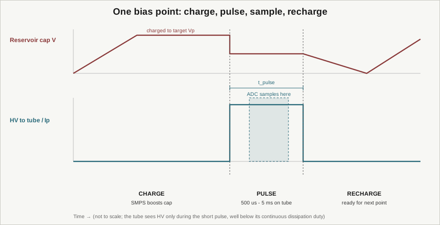
One data point on a curve is one full cycle:

1. Charge. The SMPS boosts the reservoir cap to the target plate voltage for this point. The tube sees nothing on its plate yet.
2. Pulse. The high-side switch connects the charged cap to the plate. The tube conducts; plate current flows out of the reservoir cap. This is the only interval the tube is at high voltage, and it lasts 500 µs to 5 ms, set by the micro-controller.
3. Sample. Inside that pulse window, the ADC digitizes plate current and the actual plate voltage (the cap has sagged somewhat under load, so you measure the voltage you actually applied, not the pre-pulse target).
4. Recharge. The switch opens, the tube goes dark, and the SMPS tops the cap back up for the next bias point.

The pulse width is the knob that keeps this safe for the tube. Duty cycle is low — a few-millisecond pulse followed by a recharge interval — so a tube can be driven to an instantaneous operating point above its continuous dissipation rating and still average out to a cool device. This is the single most important thing to get right about the instrument’s numbers, and it is a common mistake to picture it as a tens-of-microsecond pulse: the eTracer’s pulse is 500 µs to 5 ms — hundreds of microseconds to milliseconds, not “tens of microseconds.” The distinction is not pedantry; a tens-of-microsecond pulse and a several-millisecond pulse imply completely different reservoir-cap sizing, ADC timing, and thermal behavior.

Two rails means a twin-triode is swept “in one shot”: HV1 pulses one plate, HV2 pulses the other, on the same shared cathode and grid setup, so both halves of a 12AX7 come off the tube in a single pass rather than two separate mountings.

3.5 Sampling the pulse: the converter chain

3.5.1 The ADC

Current and voltage are captured by a 14-bit, 900 kSPS ADC. Both numbers earn their keep against the pulse timing:

• Speed. At 900 k samples/s, one sample is about 1.1 µs. Even the shortest 500 µs pulse is therefore hundreds of samples wide, and a 5 ms pulse is thousands, so the converter can sit comfortably inside the flat part of the pulse, take multiple samples, and average — settling transients at the leading edge can be skipped rather than smeared into the reading.
• Resolution. 14 bits is one part in 16,384 of full scale. Across a rail that spans a decade or more of useful plate current, that is enough resolution to resolve the low-current knee of a curve and the high-current top of the same family without changing the whole picture’s scale. In the same-era comparison that matters to Jeff’s bench, this is a genuine step up from the 10-bit converters used in the rival uTracer of the day (Vol 6) — 14 bits versus 10 is a 16× finer quantization.

Because the reservoir cap sags during the pulse, the eTracer measures the actual applied plate voltage during the sample window rather than assuming the pre-pulse target held. That is what lets a sagging pulsed source still produce a clean Vp/Ip point: you plot the current against the voltage you actually had, not the one you aimed for.

3.5.2 The heater DAC

The filament/heater voltage is set by a 12-bit DAC, so heater voltage is a software-controlled, resolvable quantity rather than a front-panel knob — 12 bits across the heater range gives fine steps, which matters when you want to sweep a tube at, say, reduced heater voltage to look at emission health, or hold an exact rated heater voltage for a repeatable measurement.

3.6 The tube-conditioning supplies

3.6.1 Heater / filament

Regulated DC, roughly 1.25–26.5 V (call it ~1.5–27 V) at 3 A, up to 30 W, at ≥85% efficiency and under 2 W dissipation at idle. The wide range spans low-voltage battery/directly-heated filaments up through the 25 V-class heaters, and the 3 A / 30 W ceiling covers the current-hungry heaters within that span. Being regulated DC (not raw AC off a transformer) it is quiet and settable, and as noted above the setpoint comes from the 12-bit DAC. One documented limitation lives here rather than in the hardware envelope: at review time the software did not compensate heater voltage for the drop caused by large heater currents (Vol 4/Vol 5) — the supply itself is specified, but the host did not correct for lead/contact drop under heavy heater load.

3.6.2 Grid bias — and the hard limit

The grid supply runs 0 to about −160…−180 V — sources quote “0 to −160 V,” “0 to −180 V,” and one review measured down to −170 V, so treat it as ≈ −160 to −180 V of available negative bias. This sets the family of grid steps that produces a curve family: the software walks the grid more negative between traces while sweeping the plate, and each trace is one grid voltage.

The hard architectural limit: there is no positive grid drive. The eTracer cannot bias the grid above 0 V. A positive-grid (“A2”) test mode exists in the software, but it is reported as unreliable and should not be counted as a real capability. For anything requiring genuine positive-grid characterization — A2 triodes, some transmitting service — this instrument is the wrong tool, and that is a design boundary, not a settings problem. The head-to-head with tracers that offer an optional positive-grid extension is Vol 6.

3.7 Power, protection, and physical envelope

3.7.1 Input power

The board runs from 29 VDC at 3 A. Standby draw is under 2 W — the SMPS chargers are idle when no pulse is pending — and the peak additional draw is about 50 W during capacitor charging, i.e. when the reservoir caps are being pumped up between bias points. The input supply therefore has to source the charging burst, not the average, which is why a full kit bundles a dedicated PSU (Vol 5). The poorly-marked PSU polarity on the PCB is a documented hazard — the silkscreen does not make polarity obvious and getting it wrong can do real damage — but that is a build/setup caution covered in Vol 5, flagged here only because it lives at this 29 VDC input.

3.7.2 Protection

The board carries over-current, over-voltage, and short-circuit protection. That is the electrical backstop for the obvious failure modes of a pulsed HV tester: a shorted or gassy tube, an internal arc, or a wiring error at the socket. It is worth being precise about what this protection is and is not — it guards the instrument against fault currents; it is not a substitute for operator HV discipline. Up to 750 V on the rails plus the energy stored in the reservoir caps is lethal, and the caps hold charge after the pulse and after power-down. The full discharge/interlock discipline is Vol 5’s subject; the hardware fact to carry from this volume is that the protection is device-protection, and the stored-energy hazard is real and independent of it.

3.7.3 Physical

The PCB is roughly 21 cm × 15 cm; the vendor’s Model-01 chassis is about 26 × 19 × 10 cm. It ships as a fully assembled, tested, and calibrated SMD board — not a solder-kit and not a publish-the-files DIY project (that commercial-assembled nature is the Vol 1/Vol 6 framing). What the buyer adds around this board — sockets, HT wire, 4 mm plugs, the chassis itself — is Vol 5.

3.8 How a single curve family comes together

Putting the pieces in sequence, a Full Scan (the scan modes themselves are Vol 4) is nothing more than this hardware cycle run in a nested loop:

1. Set the heater voltage via the 12-bit DAC and let the tube warm.
2. Pick a grid bias (0 to ≈ −160…−180 V) for the first trace.
3. For each plate-voltage point along that trace: charge the reservoir cap to the target Vp, pulse it onto the plate for 500 µs–5 ms, sample Ip and the actual Vp with the 14-bit / 900 kSPS ADC, then recharge.
4. Step the grid more negative and repeat the plate sweep for the next trace.

Each pulse is one dot; each grid step is one curve; the stack of curves is the family. The reservoir-cap architecture is what makes step 3 cheap and non-destructive, the two rails are what let a twin-triode or a pentode’s plate-and-screen be handled together, and the 14-bit/900 kSPS converter is what turns each short pulse into a point precise enough to extract gm, µ, and rp downstream in the host software (Vol 4). The hardware, in other words, does exactly one clever thing — store energy slowly, release it in a measured burst, and digitize the burst — and everything else on the board exists to set that up and read it out.