eTracer — Vol 4: Operating It

Volumes 1 through 3 covered what the eTracer is (Chris Chang / Essues Co., Ltd., Taiwan, introduced late 2017 — an independent commercial rival inspired by Dekker’s uTracer, not a Dekker design and not a member of the uTracer line), where it sits in the pulsed-HV tube-tracer landscape, and how the hardware measures. This volume is about driving it: the host software, the two scan modes, walking a triode, twin-triode and pentode through a measurement, reading the resulting curve family, and getting the data back out — including a SPICE model.

Everything below assumes the safety discipline covered in Vol 5. The two HV rails reach 0-750 V at 300 mA each and the reservoir capacitors store real energy; nothing here is casual.

4.1 The host software

The eTracer is a PC-controlled instrument — there is no front-panel graph, no knobs that set a sweep. All of the operating surface lives in a host application on the connected computer, and the board is a sequencing-and-measurement engine that the software commands.

4.1.1 What it is written in

The host is written in Python, built on the scientific stack — NumPy, SciPy and Matplotlib. That choice shows up directly in how the tool behaves: the curve plotting is Matplotlib, the numerical work (parameter extraction, spline smoothing) leans on NumPy/SciPy, and the whole thing is nominally cross-platform because Python is.

In practice the vendor packages and licenses it as a Windows application. It is used on Windows out of the box; the Python base is what makes it portable rather than any officially supported Linux build.

4.1.2 Running it on Linux under Wine

Because it is a Windows-packaged Python app rather than something tied to Windows-only APIs, it runs on Linux under Wine — the Bartola Valves build/review ran exactly that way. Read it as a Windows-packaged Python application: portable in principle, distributed for Windows in practice, and coaxed onto Linux through the compatibility layer rather than through a native package.

For Jeff’s bench that matters: the Linux-under-Wine path is a known-good option, not a gamble.

4.2 The measurement cycle you are commanding

Vol 3 covers the hardware measurement cycle and the board architecture in full — how the SMPS charges the reservoir capacitor, how the cap is switched onto the tube, how plate current is sampled, and the front-end specs (the 14-bit / 900 kSPS ADC, the 12-bit filament DAC, the 1.25-26.5 V / 3 A / 30 W heater supply). This section only recaps the one parameter of that cycle the operating software actually hands you: the pulse timing.

Per point, the tube sees a single brief HV pulse and plate current (Ip) is sampled during it, before the HV switches back off and the cap recharges for the next bias point (see Vol 3 for the full charge/pulse/sample timing). The pulse you set is 500 microseconds to 5 milliseconds — not the “tens of microseconds” you might assume from the flash-camera analogy. Because the tube only dissipates during that pulse, a scan can push it well above its continuous-dissipation rating for a single family of curves without cooking it. Every scan you set up is really a grid of these points — one charge/pulse/sample cycle per (Vp, Vg) coordinate the software walks through, and the pulse-timing setting is what governs each one.

4.3 Test modes: Full Scan vs Corners

Two modes cover the everyday work, plus a lighter scan variant.

4.3.1 Full Scan

Full Scan is the curve-tracer mode proper. The software steps the negative grid bias (Vg) through a set of fixed values, and at each grid step it walks plate voltage (Vp) up across a range, taking one pulsed Ip measurement at every step. The result is the classic family of plate-current curves: one curve per grid-bias step, Ip on the vertical axis, Vp on the horizontal. This is the data you extract gm, mu and rp from, and the data a SPICE model is fitted to.

Everything about the run is your setup: the grid-bias steps, the plate-voltage range and increment, the filament voltage, and the pulse timing. Because each point is a real HV pulse into the tube, a dense Full Scan is also the most punishing thing you can ask the tube to do — keep the plate range and grid steps inside what the tube (and the 750 V / 300 mA-per-rail envelope) can take.

4.3.2 Corners

The Corners test checks the extremes rather than filling in a whole family — it exercises the corner conditions of the operating region instead of sweeping the interior. It is the quicker, lighter-touch check: a fast way to confirm a tube is alive and behaving at the boundaries without committing to a full family of curves. Reach for it as triage; reach for Full Scan when you actually want the curves and the extracted parameters.

4.3.3 Scan variants and smoothing

The software also offers full/quick scan variants and a spline (interpolation) smoothing option that cleans up the plotted curves, plus stored measurement files you can reload. Spline smoothing is cosmetic-plus — it interpolates between measured points for a cleaner plot; the underlying samples are what they are.

4.4 Measuring a triode

The straightforward case. Set the filament voltage for the tube (via the 12-bit DAC control), wire the grid to the negative bias supply and the plate to HV1, choose Full Scan, and set:

• Filament voltage for the tube type.
• Grid-bias steps — the family of curves you want, stepping through the negative grid range (0 down to about -160 to -180 V). Note there is no positive grid drive — see the limitations section.
• Plate-voltage range and increment on HV1, inside the 0-750 V / 300 mA envelope.
• Pulse timing within the 500 microsecond - 5 millisecond window.

Run it, and you get the plate-curve family plus the extracted parameters (quiescent current, gm, mu, rp).

4.5 Measuring a twin-triode “in one shot”

The eTracer has two independent HV rails, and that is what makes a twin-triode efficient. A dual triode such as a 12AX7 can be measured “in one shot” by using the two HV supplies together — HV1 feeds one plate, HV2 feeds the second plate — so both sections are characterized in a single run rather than as two separate sessions. That is one of the standout convenience features of the two-rail design for the tubes most people actually test.

4.6 Measuring a pentode

For a tetrode or pentode, the second rail does different duty: HV1 -> plate, HV2 -> screen. You set the screen voltage on HV2 and run the plate family on HV1 exactly as for a triode, and you get the pentode’s characteristic knee’d curves.

One caution from the reviewer, carried into the limitations section below: the software does not validate pentode-mode settings for you — it will let you enter combinations it should probably question, so the sanity check is on you.

4.7 Reading the curve family

The plot is only useful if you can read it. The three small-signal parameters the host reports — transconductance (gm), amplification factor (mu), and plate resistance (rp) — each correspond to a geometric feature of the family, and the eTracer also reports the tube’s quiescent current.

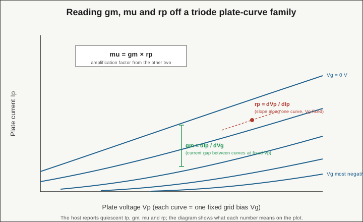
• Plate resistance rp = dVp / dIp — the slope along one curve (grid bias held fixed). A flat curve is a high rp (high output impedance); a steeply rising curve is a low rp.
• Transconductance gm = dIp / dVg — the vertical current gap between adjacent curves at a fixed plate voltage, divided by the grid-step size. Widely spaced curves mean high gm.
• Amplification factor mu = gm x rp — how far the whole family shifts horizontally per volt of grid change. It falls out of the other two.

The host does this extraction and reports the numbers, so you are not forced to read them off the graticule by eye the way you would on an analog scope-based tracer — but knowing what each one is on the plot is how you sanity-check the reported value and how you spot a tube that is soft, gassy or mismatched against its curve shape rather than a single number.

This is the whole reason a pulsed curve tracer sits on the bench next to the go/no-go testers (the Heathkit TT-1 transconductance tester and the Supreme 385 emission tester): those give you a single number and a verdict; the eTracer gives you the shape, the parameters, and something you can turn into a model.

4.8 Getting the data out

The eTracer is built to produce records, not just a glance at a screen.

4.8.1 Text, CSV, PDF and images

Measured curves and data export to text, CSV and PDF, and the curve images themselves save as JPEG or BMP. CSV is the workhorse for anything you want to re-plot or process yourself; PDF is the tidy record; the image formats are for dropping a curve into a writeup.

4.8.2 SPICE model export

The higher-value output: the eTracer can export a SPICE model of the measured tube, through Chris Chang’s conversion utility, in a form compatible with Derk Reefman’s “ExtractModel” SPICE-model extraction workflow. That closes the loop from a physical NOS or pulled tube to a simulatable device — measure the real curves, fit a model, drop it into a circuit simulation. For anyone designing or modeling tube stages, that path from bench to SPICE is the feature that justifies the instrument over a simpler tester.

4.9 Software limitations

The host does the job, but the reviewer (Bartola Valves, Jan 2018) was clear about where it is rough, and these are worth knowing before you rely on it:

• No positive grid drive. There is no positive grid supply. An A2 (positive-grid) test mode exists in the software but is reported unreliable — do not count on it for A2 characterization.
• No heater-voltage compensation for large heater currents (as of the review). High-current heaters can pull the filament voltage off its set point without the software correcting for it — relevant for big power tubes.
• Basic graphics. The plotting is functional Matplotlib, not a polished GUI.
• Cannot zoom without losing plots — and there is no drag-cursor readout on the curves. You cannot hover a point to read its value; zooming into a region drops the existing plots rather than magnifying them.
• Pentode-mode settings are not validated by the software — it will accept combinations it should arguably reject, so pentode setups need your own sanity check (as noted above).
• Thin documentation. Covered in Vol 5, but it bears repeating here: the operating documentation is thin compared to the uTracer’s, so some of the workflow is learned by doing.

None of these are fatal — this is a capable curve tracer that produces real families, real extracted parameters, and SPICE models — but they are the sharp edges to work around. The graphics and cursor limitations in particular mean the analysis comfort trails the measurement quality; the 14-bit / 900 kSPS front end is better than the software’s presentation of it.

4.10 Where this leaves the operator

Day to day, the eTracer workflow is: set the filament, pick Full Scan (or Corners for a quick check), define the grid steps and plate range inside the 0-750 V / 300 mA envelope, run the pulsed scan, read gm/mu/rp off the reported values and the curve shape, and export CSV/PDF or a Reefman-compatible SPICE model. The two rails let a twin-triode go in one shot and a pentode’s screen ride on HV2. The limits to keep in the back of your mind are no positive grid drive and a host UI whose graphics and cursor handling lag its measurement hardware.

Vol 5 covers integrating the assembled board into a chassis, the poorly-marked PSU polarity caution, calibration, the heater-compensation quirk, upkeep, and the full HV safety discipline. Vol 6 puts the eTracer head-to-head with the rival uTracer6 with a spec-and-workflow cheatsheet.