uTracer6 — Vol 3: Hardware Architecture & Measurement

3.1 The problem the hardware is built around

A tube curve tracer has to place a known plate voltage on a tube, hold a known grid bias, and read the resulting plate current — then do that again for the next point on the curve, hundreds of times, to draw a family of characteristics. The uTracer6’s design brief pushes both axes hard: plate and screen up to 1000 V, plate/screen current up to about 1 A. Held continuously, 1000 V at 1 A is 1 kW into the tube, which no tube under test would survive and no bench supply the size of this board could deliver.

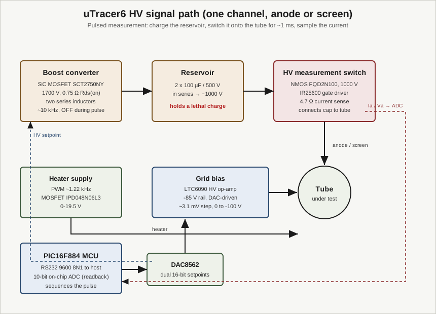
The whole uTracer line, the uTracer6 included, sidesteps that with a pulsed measurement. Small boost converters — Dekker describes each as “nothing more than an inductor, a transistor and a diode” — charge large electrolytic reservoir capacitors up to the target voltage over many milliseconds at low average power. For an actual measurement, the charged capacitor is connected to the tube through an electronic switch for a single brief pulse, roughly 1 ms long, and the plate/screen current is sampled during that window. Crucially, every switch-mode converter is switched off during the measurement pulse, so the tube sees a clean, quiet reservoir rather than a live switcher. The pulse partly discharges the reservoir; that droop is itself measured and compensated in the reported result.

The payoff is that the peak pulsed power can be about 1 kW while the average dissipation in the tube stays trivially low — the tube is only conducting for ~1 ms at a time. That is what lets a 6 x 6 in through-hole board exercise sweep tubes, beam-power tubes, and transmitter tubes at operating points a continuous supply could never reach on a hobby budget. This volume walks the signal path from the boost stage through the reservoir, the 1000 V switch, and the current sense, then covers the grid-bias and heater rails and the control core that sequences all of it.

This is a distinct kilovolt-class Dekker model, not a revision of the uTracer3 and not the current-mainstream part — the lineage and where the 6 sits are in Vol 2; building the kit and the host software are in Vol 4; operating it and its safety envelope are in Vol 5.

3.2 Charging the reservoir: the boost stage

3.2.1 The SiC boost switch

The uTracer6 has to lift a low-voltage supply rail up toward 1000 V, and it does it with a boost (step-up) converter built around two series inductors and a single switching transistor. The switching device is the piece that changes the most versus the lower-voltage uTracers: a silicon-carbide (SiC) power MOSFET, the SCT2750NY, rated 1700 V breakdown with 0.75 ohm on-resistance. Switching frequency is around 10 kHz.

Two things about that part choice are worth pulling out. First, the 1700 V rating gives real headroom over the ~1000 V reservoir target — a boost converter’s switch sees the output rail (plus ringing and margin), so a 1000 V rail wants a switch comfortably above 1000 V, and 1700 V provides that. Second, SiC is what makes a 1000 V boost stage practical on a hobbyist board at all: SiC MOSFETs hold high blocking voltage with manageable on-resistance and fast, clean switching, where a comparable silicon device would be bulkier and lossier. The 0.75 ohm Rds(on) is high by low-voltage-MOSFET standards but entirely reasonable for a 1700 V SiC part whose job is intermittent charging, not continuous heavy conduction.

The ~10 kHz switching frequency is modest on purpose. The converter only has to trickle-charge the reservoir up to setpoint between measurements; it is not delivering continuous load current, so there is no reason to run it fast and fight the switching losses and EMI that a kilovolt rail would make worse.

3.2.2 Series reservoir capacitors: two 100 uF / 500 V to reach ~1000 V

The energy for each pulse is parked in the reservoir: two 100 uF / 500 V electrolytic capacitors in series, which stacks their voltage ratings to give a reservoir good for about 1000 V. Series-stacking is the standard trick when you need a working voltage above any single affordable electrolytic’s rating — two 500 V caps in series hold ~1000 V; the tradeoff is that the series combination has half the capacitance of one, so 100 uF + 100 uF in series behaves like a single ~50 uF reservoir at ~1000 V.

That capacitance sets the droop budget. During the ~1 ms pulse the tube draws current out of the reservoir and the rail sags; the firmware measures the actual anode voltage during the pulse rather than trusting the pre-charge setpoint, so the droop is compensated rather than becoming an error. A larger reservoir would droop less but take longer to charge and store more energy; the 2 x 100 uF choice is the balance point for a 1000 V / ~1 A pulse.

It is also where the danger lives. A reservoir charged to ~1000 V holds a genuinely lethal charge — enough stored energy to hurt or kill, and it does not bleed off instantly when you power down. This volume flags that; the actual stored-energy figure, the discharge procedure, and the bench discipline around it are covered in Vol 5. Treat a powered or recently-powered uTracer6 as live at the kilovolt level.

3.3 The 1000 V switch and the current sense

3.3.1 FQD2N100 NMOS and the IR25600 driver

Between the reservoir and the tube sits the high-voltage measurement switch — the part that actually gates the pulse onto the plate (or screen). It is a 1000 V-rated N-channel MOSFET, the FQD2N100 (with the STD2NK100Z documented as an alternate), driven by an IR25600 dual gate-driver IC. A current-sense resistor of 4.7 ohm (the default value) sits in that path so the plate/screen current develops a measurable voltage across it.

The gate driver matters more than it looks. The choice of an IR25600 high-voltage gate-driver IC implies the NMOS is driven high-side of the kilovolt rail, its gate referenced to a source node that would swing up near 1000 V during the pulse. A dedicated high-voltage gate-driver IC like the IR25600 provides that level-shifted, referenced drive cleanly and fast, so the switch turns fully on for the pulse and fully off between pulses — a slow or ill-referenced gate here would waste the switch’s rating and add error to the pulse edges.

3.3.2 The 4.7 ohm current sense

Current is read as the voltage across the 4.7 ohm sense resistor. That value is a compromise: large enough to give a usable sense voltage at small plate currents, small enough not to steal much of the pulse voltage or dissipate excessively at the high end of the current range. Because the sense resistor is the default, it is one of the values a builder measuring unusual tubes might reconsider — but for the stock instrument, 4.7 ohm is what the firmware’s scaling expects, and the sensed voltage feeds back to the PIC’s on-chip ADC for the actual current reading.

3.4 The measurement pulse, step by step

Reading a single point on a curve is a short, ordered sequence, and the ordering is the whole trick:

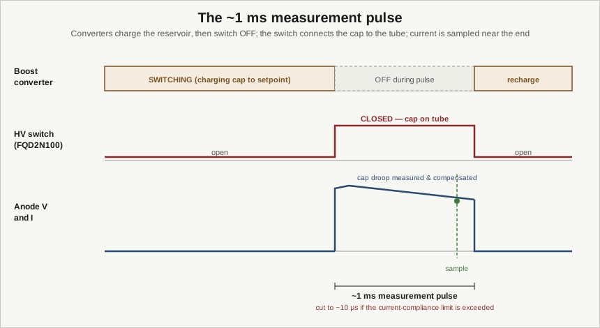
1. Charge. With the tube not yet connected to the reservoir, the boost converter runs (~10 kHz) and charges the series reservoir toward the setpoint plate/screen voltage. Grid bias and heater are already established on their own rails.
2. Quiet the converters. Just before the pulse, the switch-mode converters are turned off. The tube is about to be measured against a passive charged capacitor, not a running switcher — no switching noise contaminates the measurement.
3. Pulse. The HV switch closes, connecting the reservoir to the tube for roughly 1 ms. Plate current flows; the reservoir droops slightly; the anode voltage is measured during the pulse so the droop is accounted for.
4. Sample. Near the end of the ~1 ms window, once things have settled, the plate/screen current (via the 4.7 ohm sense) and the actual anode voltage are read by the 10-bit ADC.
5. Open and recharge. The switch opens, the tube stops conducting, and the converters come back on to recharge the reservoir for the next point.

Overlaid on that is a protection mechanism: if the current-compliance limit is exceeded, the firmware can cut the pulse short to about 10 us, aborting long before the full ~1 ms elapses, to protect the tube and the hardware from a fault or a wildly conducting device. That ~10 us fast-abort is a safety cutoff, not the normal sample time — the normal measurement pulse is ~1 ms. (There is no “faster sampling” advantage over the uTracer3 here; the uTracer6’s advance is voltage and current headroom, and the pulse is the same order of duration as the rest of the line.)

3.5 The grid-bias circuit

The grid is where the uTracer6 diverges most cleanly from the older uTracer3 approach. Instead of the uTracer3’s PWM-derived grid supply, the uTracer6 generates grid bias with a high-voltage op-amp, the LTC6090 (rated for supplies up to 140 V), running from a -85 V rail produced by an inverting boost converter. The op-amp’s input comes from the DAC, so the grid setpoint is set directly and cleanly in analog, and a potentiometer trims the offset (the grid-zero calibration, done after warm-up — see Vol 4/Vol 5).

The resolution follows from the DAC driving it: the grid-bias step works out to about 3.1 mV (100 V spread over roughly 2^15 codes). That fine a step on a 0 to -100 V range is what lets the tracer place closely-spaced grid curves and resolve a tube’s transfer characteristic near cutoff. The negative-grid range covers the normal 0 to -100 V; the optional positive-grid extension board (uTracer6-only, +100 V grid plus 0-100 mA grid-current measurement) is covered in Vol 4 — it is an add-on, not part of the base grid circuit described here.

Driving the grid from a real HV op-amp on a dedicated rail, rather than filtering a PWM, is why the grid bias is quiet and well-defined even while the plate stage is slamming kilovolt pulses a few centimetres away on the same board.

3.6 The heater supply

The heater (filament) rail is a PWM supply, ~1.22 kHz, switched directly by a MOSFET — the IPD048N06L3 — across a range of 0 to 19.5 V. The 1.22 kHz figure is a deliberate reduction from the uTracer3’s ~19.53 kHz heater PWM. Running the heater PWM slow keeps its switching activity well separated in frequency from the measurement electronics and reduces the high-frequency content coupling around a board that is already managing a kilovolt pulse; the filament’s thermal mass smooths the low-frequency PWM into a steady heating current regardless. As with the other rails, the heater is established and settled before a measurement sequence runs.

3.7 The control core

3.7.1 PIC16F884 microcontroller

Everything above is sequenced by a single Microchip PIC16F884 (the successor to the uTracer3’s PIC16F874A), and the firmware stays compatible with the uTracer3 lineage — which is why the same Windows host GUI family drives both. The host link is plain RS232, 9600 baud, 8-N-1. Everything the host asks for — set this plate voltage, this grid bias, this heater, take a point — is turned by the PIC into the charge/quiet/pulse/sample/recharge sequence, including firing the HV switch and reading back the result.

That the whole instrument runs on a modest 8-bit PIC over a 9600-baud serial line, not a fast processor or a high-speed bus, reinforces the point that the pulsed architecture does the heavy lifting: the MCU only has to time the pulse and read a handful of values per point, not stream data at high rate.

3.7.2 DAC8562 and the 10-bit ADC

Setpoints — plate/screen voltage targets and grid bias — are established with a DAC8562, a dual 16-bit DAC. (Whether every setpoint channel on the board is a full 16-bit DAC or a mix is not fully pinned down in the source material; what is clear is that the grid path resolves to about 3.1 mV, implying roughly a 15-bit effective span across the +/-100 V grid range.) The measurement readback — sensed current and actual anode voltage during the pulse — is digitized by the PIC’s on-chip 10-bit ADC.

The asymmetry there is intentional and typical of this class of instrument: you want setpoints placed finely (16-bit-class DAC resolution, hence the 3.1 mV grid step) so curves are smooth and closely spaced, but the readback only has to resolve a measured point to plotting/modelling accuracy, which a 10-bit ADC handles at the pulse rate. High readback resolution would be wasted against tube-to-tube spread and the reservoir-droop compensation anyway.

3.8 Board and construction

The uTracer6 is a 6 x 6 in (152.4 x 152.4 mm) board, larger than the uTracer3/3+‘s 4 x 6.4 in — the extra area is the HV power stage, not a re-spin of the smaller board. It is built entirely from through-hole components, which Dekker keeps deliberately “amateur-friendly”: everything is hand-solderable, with no fine-pitch surface-mount work required to assemble the kit. That through-hole choice, the single 8-bit PIC, and the “inductor, transistor, diode” converters are all of a piece — a kilovolt-class instrument that a hobbyist can actually build and repair on the bench. The assembly and calibration steps live in Vol 4.

3.9 What this architecture buys, and what it doesn’t

The pulsed, charge-then-switch design is the reason a 6 x 6 in kit can reach 1000 V and ~1 A (about 1 kW peak pulsed) without a rack of supplies and without cooking the tube — the tube conducts for ~1 ms at a time, so peak power is high while average dissipation stays low. The SiC boost switch and the series 500 V electrolytics are what push that envelope up to the kilovolt class; the LTC6090 grid circuit and the slowed heater PWM are what keep the low-level measurement quiet next to all that HV energy; and the PIC/DAC/ADC core keeps the whole thing to an 8-bit MCU and a 9600-baud serial link.

What it does not buy is speed or forgiveness. The measurement pulse is ~1 ms, the same order as the rest of the uTracer line — the advance over the uTracer3 is headroom, not sample rate. And a charged kilovolt reservoir sitting on a hobbyist through-hole board is a real hazard that does not go away at power-off, plus the higher-voltage stage is more oscillation-prone than the lower-voltage uTracers, which is why Dekker aims it at experienced builders. Operating it safely, taming oscillation, and the measurement workflow in practice are Vol 5.